Shading Intro
COS350 - Computer Graphics
Shading
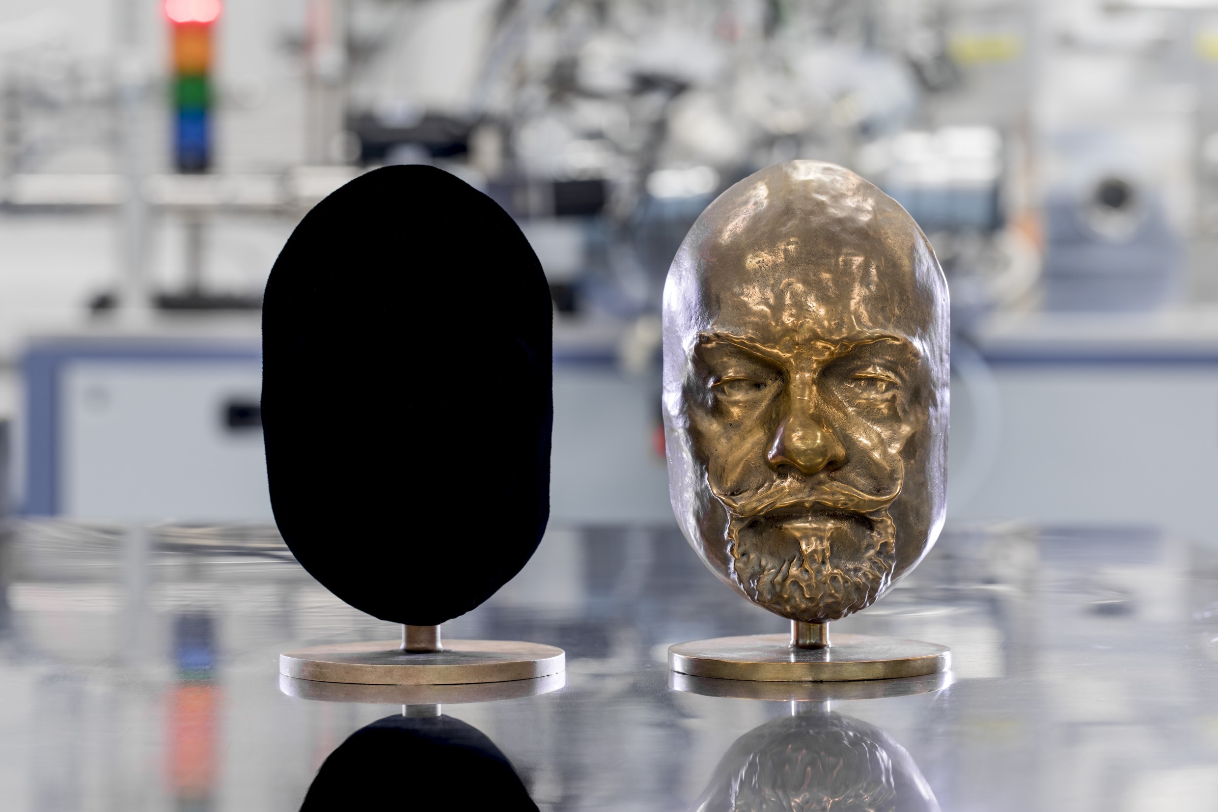
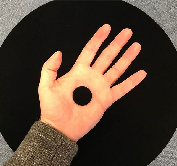
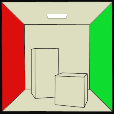
without shading, we can perceive silhouettes, but nothing else

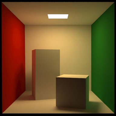
Shading
- our visual system uses variation in observed color across a surface for identification
- objects with uniform color are typically not seen in real world
- color uniformity can cause disorientation
 |
 |
Shading

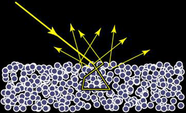
we can approximate real world by simulating light bouncing around in scene of objects with modeled materials, lighting, participating media, vision systems, etc.
\[\begin{array}{rcl} L_o(\point{x}, \omega_o) & = & L_e(\point{x}, \omega_o) + L_r(\point{x}, \omega_o) \\ L_r(\point{x}, \omega_o) & = & \int_\Omega \rho(\point{x}, \omega_i, \omega_o) L_i(\point{x}, \omega_i) (\omega_i \cdot \direction{n}) d\omega_i \end{array}\]
- compute reflected light, \(L_o\)
- depends on:
- view position: \(\point{x}\), \(\omega_o\)
- surface emitting and reflecting light: \(L_e\), \(L_r\)
- incoming light (ex: lighting): \(L_i\), \(\omega_i\)
- surface geometry and material: \(\direction{n}\), \(\rho\)
Shading
we can approximate real world by simulating light bouncing around in scene of objects with modeled materials, lighting, participating media, vision systems, etc.
\[\begin{array}{rcl} L_o(\point{x}, \omega_o) & = & L_e(\point{x}, \omega_o) + L_r(\point{x}, \omega_o) \\ L_r(\point{x}, \omega_o) & = & \int_\Omega \rho(\point{x}, \omega_i, \omega_o) L_i(\point{x}, \omega_i) (\omega_i \cdot \direction{n}) d\omega_i \end{array}\]
Note: the incoming light (\(L_i\) along \(\omega_i\)) can come:
- directly from a light source,
- or indirectly by
- bouncing off other objects in the scene or
- passing through a participating medium
Simplified rendering equation
we can approximate real world by simulating light bouncing around in scene of objects with modeled materials, lighting, participating media, vision systems, etc.
\[\begin{array}{rcl} L_o(\point{x}, \omega_o) & = & L_e(\point{x}, \omega_o) + L_r(\point{x}, \omega_o) \\ L_r(\point{x}, \omega_o) & = & \int_\Omega \rho(\point{x}, \omega_i, \omega_o) L_i(\point{x}, \omega_i) (\omega_i \cdot \direction{n}) d\omega_i \end{array}\]
we will simplify the rendering equation by ignoring \(L_e\), replace the integral with a sum, splitting reflectance into diffuse and specular, and handling indirect and reflection separately \[ c = \overbrace{\rho_d L_a}^{\text{indirect}} + \overbrace{\sum\nolimits_{i} \underbrace{(\rho_d + \rho_s)}_{\f_r} \* \underbrace{L_i \* V_i(\tilde\p)}_{L_i} \* \underbrace{| \hat\n \* \hat\l_i |}_{\omega_i \cdot \direction{n}}}^{\text{direct}} \, +\, \overbrace{k_r \ \mathrm{raytrace}(\tilde\p,\hat\r)}^{\text{reflection}} \]
shading intro
a moment for a word...
Gen 1:1–5 (ESV)
“1 In the beginning, God created the heavens and the earth. 2 The earth was without form and void, and darkness was over the face of the deep. And the Spirit of God was hovering over the face of the waters.
3 And God said, "Let there be light,"" and there was light. 4 And God saw that the light was good. And God separated the light from the darkness. 5 God called the light Day, and the darkness he called Night. And there was evening and there was morning, the first day.
”
shading intro
lighting: sources of energy (illumination)
Lighting
- determines how much light reaches a point
- depends on:
- light geometry
- light emission
- scene geometry
Light Source Models
describe how light is emitted from light sources
two categories of lighting models
- empirical light source models
- point, directional, spot
- physically-based light source models
- area light, sky model
will use empirical models in this class
Ray Tracing Lighting Model
- point/directional/spot light sources
- sharp shadows
- sharp reflection/refractions
- hacked diffuse inter-reflection: ambient term
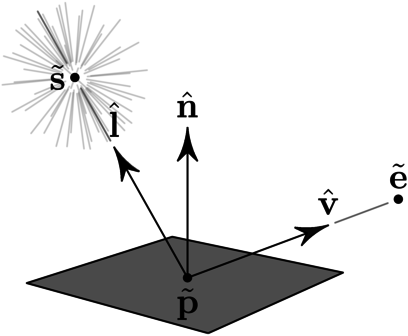
Point Lights #
- light is emitted equally from a point \(\point{s}\) in all directions
- simulate local lighting, different at each surface point \(\point{p}\)
- light direction: \(\direction{l} = \langle \point{s} - \point{p} \rangle = \frac{ \point{s} - \point{p} }{ || \point{s} - \point{p} || }\)
- light response: \(L = \frac{k_l}{|| \point{s} - \point{p} ||^2}\)
 |
|
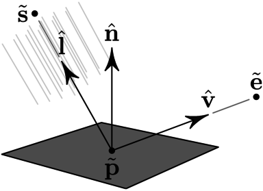
Directional Lights
- light is emitted from infinity in one direction \(\direction{d}\)
- simulate distant lighting, e.g. sun, same at all surface points \(\point{p}\)
- light direction: \(\direction{l} = \direction{d}\)
- light response: \(L = k_l\)
 |
|
Spot Lights
- same as points lights, but emits in a cone around light dir \(\hat\d\)
- simulate theatrical lights; arbitrary falloff (attentuation) model
- light direction: \(\direction{l} = \langle \point{s} - \point{p} \rangle = (\point{s} - \point{p}) / || \point{s} - \point{p} ||\)
- light response: \(L = k_l \* \mathit{attenuation}(\direction{l}; \frame{f}) / || \point{s} - \point{p} ||^2\)
 |
|
Spot Lights
Attenuation function can be arbitrary. For example,
- 1 if angle between \(\direction{l}\) and light's "forward" direction (frame \(\direction{z}\)) is less than 60°; otherwise 0
- color is some function on angle between \(\direction{l}\) and light's forward direction
- use \(\direction{l}\) wrt lighting frame to lookup color in image (ex: Gobo)

Incident Light / Cosine falloff #
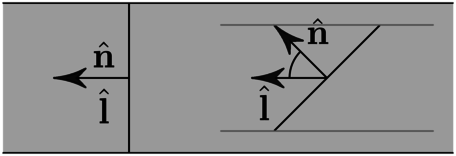
- beam of light is more spread on oblique surfaces
- incident light depends on angle
- light fraction
- infinitely thin (ex: plane): \(f = | \direction{n} \* \direction{l} |\)
- otherwise: \(f = \max(0, \direction{n} \* \direction{l})\)
 |
|
shading intro
materials: modeling how light interacts with surface
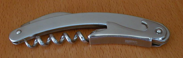
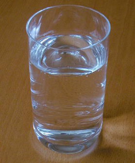
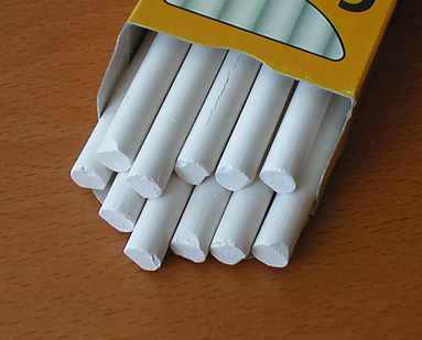
Real-World Materials
| Metals | Dielectric |
|---|---|
 |
 |
 |
 |
Real-World Materials
| Metals | Dielectric |
|---|---|
 |
 |
 |
 |
Surface Reflectance
-
surface reflectance is described by the BRDF, bidirectional reflectance distribution functions
-
BRDF is simple for simple reflactance models
-
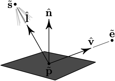
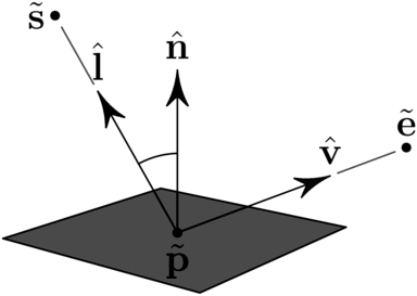
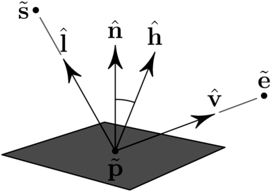
in general, the BRDF is a function of incoming and outgoing angles \(\rho(\hat\l,\hat\v;\check\f)\)
- \(\hat\l\) is the direction from the point to the light
- \(\direction{v}\) is the direction from the point to the viewer / \(\point{e}\) of ray
- \(\check\f\) is the local shading frame that describes surface orientation (normal and tangents)
Reflectance (Shading) Models
two categories of reflectance models
-
empirical models
- produce believable images
- simple and efficient
- only for simple materials
- can combine to make more complicated materials
-
physically-based shading models
- can reproduce accurate effects
- more complex and expensive
will use empirical models in this class
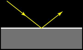
Reflectance Model
break reflectance model into two components:
-
diffuse reflection
- light is reflected in every direction equally
- colored by surface color
-
specular reflection
- light is reflected only around the mirror direction
- white for plastic-like surfaces (glossy paints)
- colored for metals (brass, copper, gold)
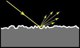
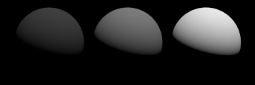
Lambert Diffuse Model #
- simple and efficient diffuse model
- produce matte appearance
- light is scattered uniformly in all directions
- brdf: \(\rho_d(\hat\l,\hat\v;\check\f) = k_d\)
 |
 |
| \(k_d\) | : | diffuse reflection intersection.material.kd |
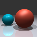
Image so far
now we can begin to understand the 3D shape of the objects, but they still look like the same material (only different color)
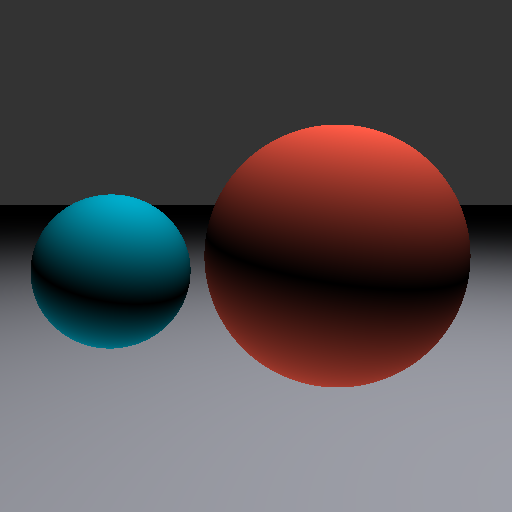 |
\[c = k_d \* L \* | \direction{n} \* \direction{l} | \]
|
why are the balls are lit from below? (will take care of this soon)
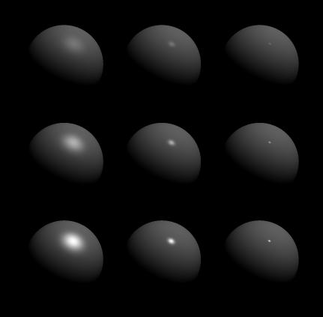
Phong specular model #
- empirical, used to look "good enough"
- produces highlight, shiny appearance
- light is scattered about the reflected light direction
- cosine of mirror \(\hat\r\) and view \(\hat\v\) direction
- reflected direction: \(\hat\r = -\hat\l + 2 (\hat\n\*\hat\l)\hat\n\)
- brdf: \(\rho_s(\hat\l,\hat\v;\check\f) = k_s \max(0,\hat\v \* \hat\r)^n\)
 |
 |
Blinn-Phong specular model #
- slightly better than Phong
- cosine of bisector \(\hat\h\) and normal \(\hat\n\)
- bisector: \(\hat\h = \langle \direction{l} + \direction{v} \rangle\)
- brdf: \(\rho_s(\hat\l,\hat\v;\check\f) = k_s \max(0,\hat\n \* \hat\h)^n\)
 |
|
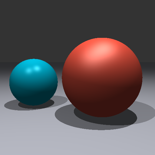
Image so far
objects appear distinct in terms of glossiness

\[c = \left( k_d + k_s \max(0,\hat\n \* \hat\h)^n \right) \* L \* | \direction{n} \* \direction{l} | \]
Reflectance Model with Multiple Lights #
when there are multiple lights, add contribution of all lights for diffuse and specular
\[c = \sum\nolimits_{i} \left( \rho_d(\hat\l_i,\hat\v;\f) + \rho_s(\hat\l_i,\hat\v;\f) \right) \* L_i \* | \hat\n \* \hat\l_i | \]
for Lambert and Phong
\[c = \sum\nolimits_{i} \left( k_d + k_s \max(0,\hat\v \* \hat\r_i)^n \right) \* L_i \* | \hat\n \* \hat\l_i | \]
for Lambert and Blinn-Phong
\[c = \sum\nolimits_{i} \left( k_d+ k_s \max(0,\hat\n \* \hat\h_i)^n \right) \* L_i \* | \hat\n \* \hat\l_i | \]
Reflectance Model with Multiple Lights #
Pseudocode for Lambert and Blinn-Phong
v_dir = -ray.dir      // view direction is opposite of ray direction
p = intersect.o       // intersection location
n_dir = intersect.n   // intersection normal

color = black
for each light {                              // assuming point light
    // compute lighting response
    s = light.o                               // light location
    l_dir = direction(s - p)                  // light direction
    l_dist = distance(s, p)                   // light distance
    L_res = light.kl / (distance * distance)  // light response
    cos_falloff = abs(dot(n_dir, l_dir))      // cosine falloff

    // compute material response
    h_dir = direction(v_dir + l_dir)
    brdf = mat.kd + mat.ks * max(0, pow(dot(n_dir, h_dir), mat.n)

    color += brdf * L_res * cos_falloff       // accumulate light
}
Image so far
the spatial relationships among the objects are difficult to discern

ex: how far above the plane are the two balls?
ex: why does light appear on top and bottom?
shading intro
illumination: patterns of light in the environment
Illumination Models
illumination models describe how light spreads in the environment
-
direct illumination
- incoming light comes directly from light sources
- other geometry can block light (shadows)
-
indirect illumination
- incoming light comes from other objects
- specular reflections (mirrors)
- diffuse inter-reflections
- caustics
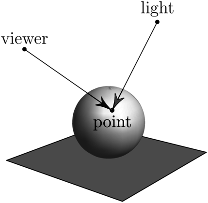
Ray Traced Shadows
- light contributes only if visible at surface point
| no shadow | shadow |
|---|---|
 |
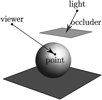 |
Ray Traced Shadows
- send a shadow ray to check if light is visible
- visible if no hits or if \(t\) more than light distance

Ray Traced Shadows #
-
shadow ray \(\point{p}_s(t) = \point{p} + t \direction{l}_i\) with \(t \in (t_{min},t_{max})\)
- spot/point light at \(\point{s}\): \(t_{max} = ||\point{s}-\point{p}||\)
- directional light: \(t_{max} = \infty\)
-
set visibility term \(V_i(\point{p})\) to...
- \(0\) if shadow ray hits something
- \(1\) if shadow ray misses everything
-
scale lighting response by visibility term \(V_i(\point{p})\)
\[c = \sum\nolimits_{i} (\rho_d + \rho_s) \* L_i \* V_i(\point{p}) \* | \direction{n} \* \direction{l}_i | \]
| \(\point{p}\) | : | intersect loc, intersect.frame.o |
| \(\direction{l}\), \(\point{s}\) | : | light direction, location (light slides) |
Image so far
it is now clear where the balls are in relation to the ground plane, but it is missing the light interaction between ground and balls

Ray Traced Shadows
implementation detail: numerical precision
- shadow acne: ray hits the same surface at the same point
- solution: only intersect if \(t > \epsilon\), i.e. \(t_{min} = \epsilon\), where \(\epsilon = 10^{-5}\)
 |
|
| \(t_{min} = 0\) | \(t_{min} = \epsilon\) |
Indirect illumination
- light bounces in environment
- ceilings are not black
- shadows are not perfectly black
- very expensive to compute all bounces
 |
 |
Ambient Term Hack #
for now, approx (poorly) diffuse reflections with a constant term
\[c = \rho_d L_a + \sum\nolimits_{i} (\rho_d + \rho_s) \* L_i \* V_i(\point{p}) \* | \direction{n} \* \direction{l}_i |\]
 |
|
Important
the ambient term is outside the sum!
Ray Traced Reflections
- "shiny" surfaces reflects light around reflected direction
- recursively trace a ray if material is reflective or refractive

Ray Traced Reflections #
- simple reflections
- along mirror direction: \(\hat\r = -\hat\v + 2(\hat\v \* \hat\n)\hat\n\)
- color sample is scaled by \(k_r\)
- implementation detail: recursion
- avoid hitting visible point: \(t_{min} > \epsilon\)
- make sure you do not recurse indefinitely!
\[\begin{array}{rcl} c & = & \rho_d L_a + \left( \sum\nolimits_{i} (\rho_d + \rho_s) \* L_i \* V_i(\tilde\p) \* | \hat\n \* \hat\l_i |\, \right) + \\ & & \qquad+\, k_r \ \mathrm{irradiance}(\tilde\p,\hat\r) \end{array}\]
Image so far

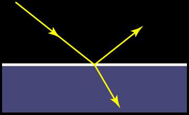
ray traced refractions
- transmissive surfaces transmit light through the surface
- transmitted light is "bent" or refracted due to changes in speed of light
- simple refractions
- along refraction direction: use Snell's Law
- see slide Appendix A for details
- color sample is scaled by \(k_t\)
\[\begin{array}{rcl} c & = & \rho_d L_a + \left( \sum\nolimits_{i} (\rho_d + \rho_s) \* L_i \* V_i(\tilde\p) \* | \hat\n \* \hat\l_i |\, \right) + \\ & & \qquad+\, k_r \ \mathrm{irradiance}(\tilde\p,\hat\r) + k_t \ \mathrm{irradiance}(\tilde\p,\hat\t) \end{array}\]
shading intro
Antialiasing
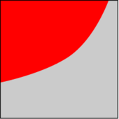
Antialiasing: removing jaggies
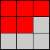
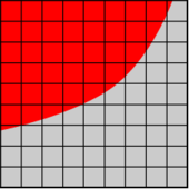
aliasing artifacts appear as jagged or saw-toothed due to under-sampling a curved shape

Antialiasing: removing jaggies
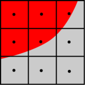
poor-man antialiasing:
- for each pixel
- take multiple samples
- compute average
Ray tracing pseudocode
original code with one sample per pixel
\[u = \frac{x + 0.5}{w} \qquad v = 1 - \frac{y + 0.5}{h} \]
for each pixel {
    determine viewing direction
    intersect ray with scene
    compute illumination
    store results in pixel
}
Anti-aliased Ray tracing pseudocode #
updated code with multiple samples per pixel
\[u = \frac{x + (i + 0.5)/s}{w} \qquad v = 1 - \frac{y + (j + 0.5)/s}{h} \]
for each pixel {
    initialize color to black
    for each sample {  // note: numberOfSamples along x and along y
        determine viewing direction based on pixel and sub-pixel sample
        intersect ray with scene
        compute illumination
        accumulate result in color
    }
    store color / numberOfSamples^2 in pixel
}
Note: numberOfSamples (\(s\)) is per dimension, so the total number of samples per pixel is numberOfSamples squared (\(s^2\)), because images are two dimensional
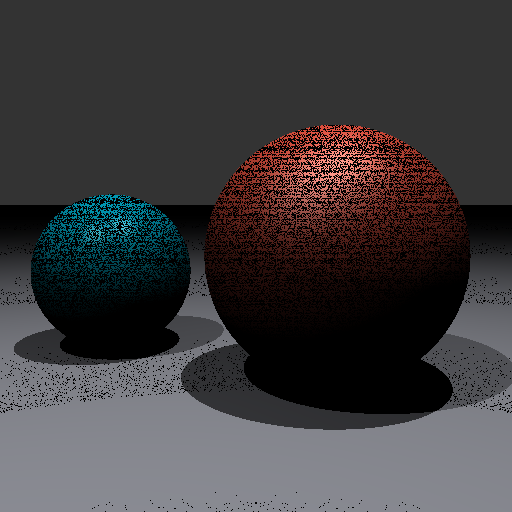
image so far


shading intro
appendices
Appendix a: Snell's Law for refraction #
Light travels slower through a medium than through a vacuum. We capture this slowness by the index of refraction equation \(n = \frac{c}{v}\), where \(c\) is speed of light in a vacuum and \(v\) is speed of light in the medium. Note: good approximations for a few media are:
| \(n\) | medium | \(n\) | medium | |
|---|---|---|---|---|
| 1.0 | air | 1.3 | water | |
| 1.5 | glass | 2.4 | diamond |
Light follows a straight line when traveling in a single medium (ignoring general relativity). However, when light transitions from one medium to another with a different \(n\), the path bends at the interface. The amount of bend is modeled by Snell's Law:
|
\[ n_1 \sin \theta_1 = n_2 \sin \theta_2 \] |
\[ \qquad \frac{\sin \theta_1}{\sin \theta_2} = \frac{n_2}{n_1} \qquad \] |
Appendix a: Snell's Law for refraction
compute the direction of transmitted light using these equations:
|
\[\begin{array}{rcl} \eta & = & \frac{n_\textit{from}}{n_\textit{to}} \\ c_1 & = & \hat\n \cdot \hat\v \\ c_2 & = & \sqrt{1 - \eta^2 (1 - c_1^2)} \\ \hat\t & = & -\eta \hat\v - (\eta c_1 + c_2) \hat\n \end{array}\] |
|
Note: total internal reflection if \(\eta^2 (1-c_1^2) \geq 1\) (expression under square root for \(c_2\) is negative!)
appendix b: fresnel #
Transparent objects, such as glass or water, are both refractive and reflective. How much light they reflect vs the amount they transmit actually depends on the angle of incidence. The amount of transmitted light increases when the angle of incidence decreases.
We can compute the ratio of reflected (\(F_R\)) vs. refracted / transmitted (\(F_T\)) light using the Fresnel equations.
\[\begin{array}{rcl} F_{R\parallel} & = & \left(\frac{n_\textit{to} \cos \theta_1 - n_\textit{from} \cos \theta_2}{n_\textit{to} \cos\theta_1 + n_\textit{from}\cos\theta_2}\right)^2 \\ F_{R\bot} & = & \left(\frac{n_\textit{from}\cos\theta_2 - n_\textit{to}\cos\theta_1}{n_\textit{from}\cos\theta_2 + n_\textit{to}\cos\theta_1}\right)^2 \\ F_R & = & \frac{1}{2}\left( F_{R\parallel} + F_{R\bot} \right) \\ F_T & = & 1 - F_R \end{array}\]
appendix c: rendering equation #
The central idea of this course is captured in one simple equation.
\[ L_o(\point{x}, \direction{\omega_o}) = L_e(\point{x}, \direction{\omega_o}) + \int_\Omega \rho(\point{x}, \direction{\omega_i}, \direction{\omega_o}) L_i(\point{x}, \direction{\omega_i}) (\direction{\omega_i} \cdot \direction{n}) d\omega_i \]
- \(L_o\) is the amount of light leaving a point \(\point{x}\) in \(\omega_o\) direction.
- \(L_e\) is the amount of light emitted from \(\point{x}\) along \(\omega_o\)
- \(\rho\) computes proportion of light reflected from \(\omega_i\) to \(\omega_o\) at \(\point{x}\)
- \(L_i\) is amount of light coming in toward \(\point{x}\) along \(\omega_i\)
- \(\direction{n}\) is direction perpendicular to surface at \(\point{x}\)
- \(\Omega\) is unit hemisphere centered around \(\point{x}\) oriented along \(\direction{n}\)