Greedy Algorithms
COS 320 - Algorithm Design
Greedy Algorithms
Coin Changing
coin changing

coin changing
Goal: Given U.S. currency denominations (\(\{1, 5, 10, 25, 100\}\)), devise a method to pay amount to customer using fewest coins.
Ex: 34¢
 |
 |
 |
|
|
|
Cashier's Algorithm: At each iteration, add coin of the largest value that does not take us past the amount to be paid.
Ex: $2.89
 |
 |
|
|
|
 |
|
|
|
|
cashier's algorithm
At each iteration, add coin of the largest value that does not take us past the amount to be paid.
Cashiers-Algorithm (x, c1, c2, ..., cn)
    Sort n coin denominations so that 0 < c1 < c2 < ... < cn.
    S <- { }  // multiset of coins selected
    While x > 0
        k <- largest coin denomination ck such that ck <= x
        If no such k
            Return "no solution"
        Else
            x <- x - ck
            S <- S | { k };
    Return S
quiz 1: greedy algorithms
Is the cashier's algorithm optimal?
-
Yes, greedy algorithms are always optimal
-
Yes, for any set of coin denominations \(c_1 < c_2 < \ldots < c_n\) provided \(c_1 = 1\)
-
Yes, because of special properties of U.S. coin denominations
-
No.

Cashier's algorithm (for arbitrary coin denominations)
Q. Is Cashier's algorithm optimal for any set of denominations?
- No. Consider U.S. postage: 1, 10, 21, 34, 70, 100, 350, 1225, 1500.
- Cashier's algorithm: 140¢ = 100 + 34 + 1 + 1 + 1 + 1 + 1 + 1
- Optimal: 140¢ = 70 + 70
 |
 |
 |
 |
 |
 |
 |
 |
 |
- No. It may not even lead to a feasible solution if \(c_1 > 1\): 7,8,9
- Cashier's algorithm: 15¢ = 9 + ?
- Optimal: 15¢ = 7 + 8
properties of any optimal solution (U.S. coin denominations)
Property: Number of pennies ≤ 4
Pf: Replace 5 pennies with 1 nickel
Property: Number of nickels ≤ 1
Property: Number of quarters ≤ 3
Property: Number of nickels + number of dimes ≤ 2
Pf:
- Recall: ≤ 1 nickel
- Replace 3 dimes and 0 nickels with 1 quarter and 1 nickel
- Replace 2 dimes and 1 nickel with 1 quarter
|
|
|
|
|
properties of any optimal solution (U.S. coin denominations)
Theorem: Cashier's Algorithm is optimal for U.S. coins {1,5,10,25,100}
Pf: (by induction on amount to be paid \(x\))
- Consider optimal way to change \(c_k \leq x < c_{k+1}\): greedy takes coin \(k\)
- We claim that any optimal solution must take coin \(k\)
- If not, it needs enough coins of type \(c_1, \ldots, c_{k-1}\) to add up to \(x\)
- Following table indicates no optimal solution can do this
- Problem reduces to coin-changing \(x-c_k\) cents, which, by induction, is optimally solved by cashier's algorithm. ∎
properties of any optimal solution (U.S. coin denominations)
| \(k\) | \(c_k\) | all optimal solutions must satisfy | max value of coin denominations \(c_1,c_2,\ldots,c_{k-1}\) in any optimal solution |
|---|---|---|---|
| 1 | 1 | \(P \leq 4\) | — |
| 2 | 5 | \(N \leq 1\) | \(4c_1 = 4\) |
| 3 | 10 | \(N + D \leq 2\) | \(1c_2 + 4c_1 = 5 + 4 = 9\) |
| 4 | 25 | \(Q \leq 3\) | \(2c_2 + 4c_1 = 20 + 4 = 24\) |
| 5 | 100 | no limit | \(3c_3 + 2c_2 + 4c_1 = 75 + 20 + 4 = 99\) |
Greedy Algorithms
Interval Scheduling (4.1)
interval scheduling
- Job \(j\) starts at \(s_j\) and finishes at \(f_j\)
- Two jobs are compatible if they don't overlap
- Goal: find maximum subset of mutually compatible jobs
: : : : : : : : : : : : : : : : : : : : : : : : : : : : : : : : : : : : : : : : : : : : : : : : : : : : : : : : : : : : : : : : : : : : : : : : : : : : : :
Example: jobs d and g are incompatible
quiz 2: greedy algorithms
Consider jobs in some order, taking each job provided it's compatible with the ones already taken. Which rule is optimal?
-
Consider jobs in ascending order of \(s_j\) (earliest start time)
-
Consider jobs in ascending order of \(f_j\) (earliest finish time)
-
Consider jobs in ascending order of \(f_j-s_j\) (shortest interval)
-
None of the above
interval scheduling: earliest-finish-time-first algorithm
Earliest-Finish-Time-First (n, s1, s2, ..., sn, f1, f2, ..., fn)
    Sort jobs by finish times and renumber so that f1 ≤ f2 ≤ ... ≤ fn
    S <- { }     // set of jobs selected
    For j = 1 to n
        If job j is compatible with S
            S <- S | { j }
    Return S
Proposition: Can implement earliest-finish-time-first in \(O(n \log n)\) time.
- Keep track of job \(j^*\) that was added last to \(S\)
- Job \(j\) is compatible with \(S\) iff \(s_j \geq f_{j^*}\)
- Sorting by finish time takes \(O(n \log n)\) time
group: interval scheduling
Earliest-Finish-Time-First (n, s1, s2, ..., sn, f1, f2, ..., fn)
    Sort jobs by finish times and renumber so that f1 ≤ f2 ≤ ... ≤ fn
    S <- { }     // set of jobs selected
    For j = 1 to n
        If job j is compatible with S
            S <- S | { j }
    Return S
interval scheduling: earliest-finish-time-first algorithm
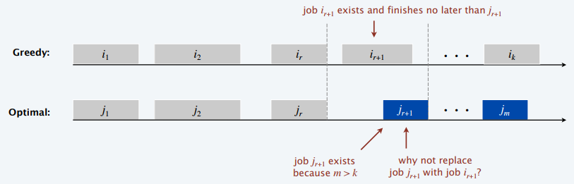
Theorem: The earliest-finish-time-first algorithm is optimal
Pf: (by contradiction)
- Assume greedy is not optimal (\(m>k\)), and let's see what happens
- Let \(i_1,i_2,\ldots,i_k\) denote set of jobs selected by greedy
- Let \(j_1,j_2,\ldots,j_m\) denote set of jobs in an optimal solution with \(i_1=j_1, i_2=j_2, \ldots, i_r=j_r\) for the largest possible value of \(r\)
interval scheduling: earliest-finish-time-first algorithm
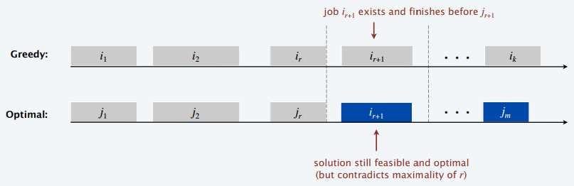
Theorem: The earliest-finish-time-first algorithm is optimal
Pf: (by contradiction)
- Assume greedy is not optimal (\(m>k\)), and let's see what happens
- Let \(i_1,i_2,\ldots,i_k\) denote set of jobs selected by greedy
- Let \(j_1,j_2,\ldots,j_m\) denote set of jobs in an optimal solution with \(i_1=j_1, i_2=j_2, \ldots, i_r=j_r\) for the largest possible value of \(r\)
quiz 3: greedy algorithms
Suppose that each job also has a positive weight and the goal is to find a maximum weight subset of mutually compatible intervals. Is the earliest-finish-time-first algorithm still optimal?
-
Yes, because greedy algorithms are always optimal
-
Yes, because the same proof of correctness is valid
-
No, because the same proof of correctness is no longer valid
-
No, because you could assign a huge weight to a job that overlaps the job with the earliest finish time
Greedy Algorithms
Interval Partitioning (4.1)
interval partitioning
Scheduling lectures to classrooms
- Lecture \(j\) starts at \(s_j\) and finishes at \(f_j\)
- Goal: find minimum number of classrooms to schedule all lectures so that no two lectures occur at the same time in the same room
Ex: This schedule uses 4 classrooms to schedule 10 lectures.
: : : : : : : : : : : : : : : : : : : : : : : : :
Example: jobs e and g are incompatible
interval partitioning
Scheduling lectures to classrooms
- Lecture \(j\) starts at \(s_j\) and finishes at \(f_j\)
- Goal: find minimum number of classrooms to schedule all lectures so that no two lectures occur at the same time in the same room
Ex: This schedule uses 3 classrooms to schedule 10 lectures.
: : : : : : : : : : : : : : : : : : : : : : : : :
Note: intervals are open, so e and h do not intersect. Need only 3 classrooms at 14:00.
quiz 4: greedy algorithms
Consider lectures in some order, assigning each lecture to first available classroom (opening a new classroom if none is available). Which rule is optimal?
-
Consider lectures in ascending order of \(s_j\) (earliest start time)
-
Consider lectures in ascending order of \(f_j\) (earliest finish time)
-
Consider lectures in ascending order of \(f_j - s_j\) (shortest interval)
-
None of the above
interval partitioning: earliest-start-time-first algorithm
// consider lectures in order of start time:
// - assign next lecture to any compatible classroom (if one exists)
// - otherwise, open up a new classroom
Earliest-Start-Time-First (n, s1, s2, ..., sn, f1, f2, ..., fn)
    Sort lectures by start times and renumber so that s1 ≤ s2 ≤ ... ≤ sn
    d <- 0     // number of allocated classrooms
    For j = 1 to n
        If lecture j is compatible with some classroom k
            Schedule lecture j in any such classroom k
        Else
            Allocate a new classroom d+1
            Schedule lecture j in classroom d+1
            d <- d + 1
    Return schedule
group: interval partitioning
interval partitioning: earliest-start-time-first algorithm
Proposition: The earliest-start-time-first algorithm can be implemented in \(O(n \log n)\) time.
Pf: Store classrooms in a priority queue (key = finish time of its last lecture)
- To determine whether lecture \(j\) is compatible with some classroom, compare \(s_j\) to key of min classroom \(k\) in priority queue.
- To add lecture \(j\) to classroom \(k\), increase key of classroom \(k\) to \(f_j\)
- Total number of priority queue operations is \(O(n)\)
- Sorting by start times takes \(O(n \log n)\) time. ∎
Remark: This implementation chooses a classroom \(k\) whose finish time of its last lecture is the earliest
interval partitioning: lower bound on optimal solution
The depth of a set of open intervals is the maximum number of intervals that contain any given point.
Key observation: Number of classrooms needed ≥ depth
Q. Does minimum number of classrooms needed always equal depth?
- Yes! Moreover, earliest-start-time-first algorithm finds a schedule whose number of classrooms equals the depth.
: : : : : : : : : :
interval partitioning: analysis of earliest-start-time-first algorithm
Observation: the earliest-start-time-first algorithm never schedules two incompatible lectures in the same classroom.
Theorem: Earliest-start-time-first algorithm is optimal.
Pf:
- Let \(d =\) number of classrooms that the algorithm allocates
- Classroom \(d\) is opened because we needed to schedule a lecture, say \(j\), that is incompatible with a lecture in each of \(d-1\) other classrooms.
- Thus, these \(d\) lectures each end after \(s_j\)
- Since we sorted by start time, each of these incompatible lectures start no later than \(s_j\)
- Thus, we have \(d\) lectures overlapping at time \(s_j + \epsilon\)
- Key observation ⇒ all schedules use \(\geq d\) classrooms. ∎
Greedy Algorithms
Scheduling to minimize lateness (4.2)
Scheduling to minimize lateness
- Single resource processes one job at a time
- Job \(j\) requires \(t_j\) units of processing time and is due at time \(d_j\)
- If \(j\) starts at time \(s_j\), it finishes at time \(f_j=s_j+t_j\)
- Lateness: \(\mathcal{l}_j = \max \{ 0, f_j-d_j \}\)
- Goal: Schedule all jobs to minimize maximum lateness \(L = \max_j \mathcal{l}_j\)
| 1 | 2 | 3 | 4 | 5 | 6 | |
|---|---|---|---|---|---|---|
| \(t_j\) | 3 | 2 | 1 | 4 | 3 | 2 |
| \(d_j\) | 6 | 8 | 9 | 9 | 14 | 15 |
:
Example: \(j_1\) has \(d_1=6\), \(f_1=8\), and lateness of \(8-6=2\), and
\(j_4\) has \(d_4=9\), \(f_4=15\), and lateness of \(15-9=6\), so maximum lateness \(L = \max \{2, 6\} = 6\)
quiz 5: Greedy Algorithms
Schedule jobs according to some natural order. Which order minimizes the maximum lateness?
-
Ascending order of processing time \(t_j\) (shortest processing time)
-
Ascending order of deadline \(d_j\) (earliest deadline first)
-
Ascending order of slack: \(d_j - t_j\) (smallest slack)
-
None of the above
minimizing lateness: earliest deadline first
Earliest-Deadline-First (n, t1, t2, ..., tn, d1, d2, ..., dn)
    Sort jobs by due times and renumber so that d1 ≤ d2 ≤ ... ≤ dn
    t <- 0
    For j = 1 to n
        Assign job j to interval [t, t + tj]
        sj <- t; fj <- t + tj
        t <- t + tj
    Return intervals [s1, f1], [s2, f2], ..., [sn, fn]
| 1 | 2 | 3 | 4 | 5 | 6 | |
|---|---|---|---|---|---|---|
| \(t_j\) | 3 | 2 | 1 | 4 | 3 | 2 |
| \(d_j\) | 6 | 8 | 9 | 9 | 14 | 15 |
:
Note: \(d_4\) has lateness of 1, so \(L = 1\)
minimizing lateness: no idle time
Observation 1: There exists an optimal schedule with no idle time.
an optimal schedule : : : :
an optimal schedule with no idle time : : : :
Observation 2: The earliest-deadline-first schedule has no idle time.
minimizing lateness: inversions
Given a schedule \(S\), an inversion is a pair of jobs \(i\) and \(j\) such that \(i < j\) but \(j\) is scheduled before \(i\).
a schedule with an inversion (i < j) :
Recall: we assume the jobs are numbered so that \(d_1 \leq d_2 \leq \ldots \leq d_n\)
Observation 3: The earliest-deadline-first schedule is the unique idle-free schedule with no inversions.
:
minimizing lateness: inversions
Observation 4: If an idle-free schedule has an inversion, then it has an adjacent inversion (two inverted jobs scheduled consecutively)
Pf:
- Let \(i\)-\(j\) be a closest inversion.
- Let \(k\) be element immediately to the right of \(j\).
- Case 1: \(k = i\), then \(i\) is adjacent to \(j\).
- Case 2: \(j > k\), then \(j\)-\(k\) is an adjacent inversion.
- Case 3: \(j < k\), then \(i\)-\(k\) is a closer inversion since \(i < j < k\). ∎
:
minimizing lateness: inversions
before exchange :
after exchange :
Key claim: Exchanging two adjacent, inverted jobs \(i\) and \(j\) reduces the number of inversions by 1 and does not increase the max lateness.
minimizing lateness: inversions
Key claim: Exchanging two adjacent, inverted jobs \(i\) and \(j\) reduces the number of inversions by 1 and does not increase the max lateness.
Pf: Let \(\mathcal{l}\) be the lateness before the swap, and let \(\mathcal{l}'\) be it afterwards.
- \(\mathcal{l}_k' = \mathcal{l}_k\) for all \(k \neq i,j\).
- \(\mathcal{l}_i' \leq \mathcal{l}_i\)
- If job \(j\) is late, \[\begin{array}{rclll} \mathcal{l}_j' & = & f_j' - d_j & \quad & \text{definition} \\ & = & f_i - d_j & & j\text{ now finishes at time }f_i \\ & \leq & f_i - d_i & & i<j \Rightarrow d_i \leq d_j \\ & \leq & \mathcal{l}_i & & \text{definition} \quad\blacksquare \end{array} \]
minimizing lateness: analysis of earliest-deadline-first algorithm
Theorem: The earliest-deadline-first schedule \(S\) is optimal
Pf (by contradiction): Define \(S^*\) to be an optimal schedule with the fewest inversions (optimal schedule can have inversions).
- Can assume \(S^*\) has no idle time (observation 1)
- Case 1: \(S^*\) has no inversions, then \(S = S^*\) (observation 3)
- Case 2: \(S^*\) has an inversion,
- let \(i\)-\(j\) be an adjacent inversion (observation 4)
- exchanging jobs \(i\) and \(j\) decreases the number of inversions by 1 without increasing the max lateness (key claim)
- contradicts "fewest inversions" part of the definition of \(S^*\) ∎
greedy analysis strategies
Greedy algorithm stays ahead:
- Show that after each step of the greedy algorithm, its solution is at least as good as any other algorithm's.
Structural:
- Discover a simple "structural" bound asserting that every possible solution must have a certain value. Then show that your algorithm always achieves this bound.
Exchange argument:
- Gradually transform any solution to the one found by the greedy algorithm without hurting its quality.
greedy algorithms
Other greedy algorithms:
- Gale-Shapley: unmatched hospital makes proposal to next student on descending preference list, students only "trade-up"
- Kruskal: in increasing order of weight, add edge if it does not make cycle
- Dijkstra: in increasing accumulated weight from source, add edge if it does not make cycle
- Prim: add minimum edge from tree to unconnected vertex
- Huffman: with each binary tree leaf as weighted by appearance frequency, create a parent node for two smallest weighted nodes having sum weight
- ...
Greedy Algorithms
Google's Foo.bar challenge
Group: Google's Foo.bar challenge
A "secret" web tool that Google uses to recruit developers.
- Triggered by specific searches related to programming.
- Algorithmic coding challenges of increasing difficulty.

Quantum antimatter fuel comes in small pellets, which is convenient since
the many moving parts of the LAMBCHOP each need to be fed fuel one pellet
at a time.  However, minions dump pellets in bulk into the fuel intake.
You need to figure out the most efficient way to sort and shift the
pellets down to a single pellet at a time.

The fuel control mechanisms have 3 operations:
 -  Add 1 fuel pellet
 -  Remove 1 fuel pellet
 -  Divide the entire group of fuel pellets by 2 (due to the destructive
    energy released when a quantum antimatter pellet is cut in half, the
    safety controls will only allow this to happen if there is an even
    number of pellets)

Write a function called answer(n) which takes a positive integer n as a
string and returns the minimum number of operations needed to transform
the number of pellets to 1.

Greedy Algorithms
optimal caching (4.3)
optimal caching
Caching
- Cache with capacity to store \(k\) items
- Sequence of \(m\) item requests \(d_1, d_2, \ldots, d_m\)
- Cache hit: item in cache when requested
- Cache miss: item not in cache when requested
- must evict some item from cache and bring requested item into cache
Applications: CPU, RAM, hard drive, web, browser, ...
Goal: Eviction schedule that minimizes the number of evictions
optimal caching
Ex: \(k=2\), initial cache \(= ab\), requests: \(a, b, c, b, c, a, b\)
Optimal eviction schedule: 2 evictions
| cache | ||
|---|---|---|
| a | a | b |
| b | a | b |
| c | a | c |
| b | b | c |
| c | b | c |
| a | b | a |
| b | b | a |
Note
Red highlight on cache miss (eviction)
optimal offline caching: greedy algorithms
LIFO/FIFO
- Evict item brought in most/least recently
LRU
- Evict item whose most recent access was earliest (least recently used)
LFU
- Evict item that was least frequently requested
optimal offline caching: greedy algorithms
LIFO: Evict item brought in most recently (stack)
optimal offline caching: greedy algorithms
FIFO: Evict item brought in least recently (queue)
optimal offline caching: greedy algorithms
LRU: Evict item whose most recent access was earliest
optimal offline caching: greedy algorithms
LFU: Evict item that was least frequently requested
optimal offline caching: farthest-in-future
Farthest-in-future algorithm evicts item in the cache that is not requested until farthest in the future (clairvoyant algorithm)
Theorem [Bélády 1966]: FF is optimal eviction schedule
Pf: Algorithm and theorem are intuitive; proof is subtle.
optimal offline caching: farthest-in-future
Farthest-in-future algorithm evicts item in the cache that is not requested until farthest in the future (clairvoyant algorithm)
quiz 6: greedy algorithms
|
Which item will be evicted next using farthest-in-future schedule?
|
| |||||||||||||||||||||||||||||||||||||||||||||||||||||||
reduced eviction schedules
A reduced schedule is a schedule that brings an item \(d\) into the cache in step \(j\) only if there is a request for \(d\) in step \(j\) and \(d\) is not already in the cache.
|
an unreduced schedule:
|
a reduced schedule:
| ||||||||||||||||||||||||||||||||||||||||||||||||||||||||||||||||||||||||||||||||
reduced eviction schedules
Claim: Given any unreduced schedule \(S\), can transform it into a reduced schedule \(S'\) with no more evictions.
Pf by induction on number of steps \(j\):
- Suppose \(S\) brings \(d\) into the cache in step \(j\) without a request
- Let \(c\) be the item \(S\) evicts when it brings \(d\) into the cache
- Case 1: \(S\) brings \(d\) into the cache in step \(j\) without a request
- Case 1a: \(d\) evicted before next request for \(d\)
- ...
reduced eviction schedules
|
unreduced schedule \(S\):
|
schedule \(S'\):
| ||||||||||||||||||||||||||||||||||||||||||||||||||||||||||||||||||||||||
- \(d\) enters cache without a request
- \(d\) evicted before next request for \(d\)
- might as well leave \(c\) in cache until \(d\) is evicted
reduced eviction schedules
Claim: Given any unreduced schedule \(S\), can transform it into a reduced schedule \(S'\) with no more evictions.
Pf by induction on number of steps \(j\):
- Suppose \(S\) brings \(d\) into the cache in step \(j\) without a request
- Let \(c\) be the item \(S\) evicts when it brings \(d\) into the cache
- Case 1: \(S\) brings \(d\) into the cache in step \(j\) without a request
- Case 1a: \(d\) evicted before next request for \(d\)
- Case 1b: next request for \(d\) occurs before \(d\) is evicted
- ...
reduced eviction schedules
|
unreduced schedule \(S\):
|
schedule \(S'\):
| ||||||||||||||||||||||||||||||||||||||||||||||||||||||||||||||||||||||||
- \(d\) enters cache without a request
- \(d\) still in cache before next request for \(d\)
- might as well leave \(c\) in cache until \(d\) is requested
reduced eviction schedules
Claim: Given any unreduced schedule \(S\), can transform it into a reduced schedule \(S'\) with no more evictions.
Pf by induction on number of steps \(j\):
- Suppose \(S\) brings \(d\) into the cache in step \(j\) without a request
- Let \(c\) be the item \(S\) evicts when it brings \(d\) into the cache
- Case 1: \(S\) brings \(d\) into the cache in step \(j\) without a request
- Case 2: \(S\) brings \(d\) into the cache in step \(j\) even though \(d\) is in cache
- Case 2a: \(d\) evicted before it is needed
- ...
reduced eviction schedules
|
unreduced schedule \(S\):
|
schedule \(S'\):
| ||||||||||||||||||||||||||||||||||||||||||||||||||||||||||||||||||||||||
- \(d\) enters cache even though \(d\) is already in cache (not necessary)
- might as well leave \(c\) in cache until \(d\) is evicted
reduced eviction schedules
Claim: Given any unreduced schedule \(S\), can transform it into a reduced schedule \(S'\) with no more evictions.
Pf by induction on number of steps \(j\):
- Suppose \(S\) brings \(d\) into the cache in step \(j\) without a request
- Let \(c\) be the item \(S\) evicts when it brings \(d\) into the cache
- Case 1: \(S\) brings \(d\) into the cache in step \(j\) without a request
- Case 2: \(S\) brings \(d\) into the cache in step \(j\) even though \(d\) is in cache
- Case 2a: \(d\) evicted before it is needed
- Case 2b: \(d\) is needed before it is evicted
reduced eviction schedules
|
unreduced schedule \(S\):
|
schedule \(S'\):
| ||||||||||||||||||||||||||||||||||||||||||||||||||||||||||||||||||||||||
- \(d\) enters cache even though \(d\) is already in cache (not necessary)
- might as well leave \(c\) in cache until \(d\) is needed
reduced eviction schedules
Claim: Given any unreduced schedule \(S\), can transform it into a reduced schedule \(S'\) with no more evictions.
Pf by induction on number of steps \(j\):
- Suppose \(S\) brings \(d\) into the cache in step \(j\) without a request
- Let \(c\) be the item \(S\) evicts when it brings \(d\) into the cache
- Case 1: \(S\) brings \(d\) into the cache in step \(j\) without a request
- Case 2: \(S\) brings \(d\) into the cache in step \(j\) even though \(d\) is in cache
- If multiple unreduced items in step \(j\), apply each one in turn, dealing with Case 1 before Case 2
- Resolving Case 1 might trigger Case 2 ∎
farthest-in-future analysis
Theorem: FF is optimal eviction algorithm
Pf: Follows directly from the following invariant
Invariant: There exists an optimal reduced schedule \(S\) that has the same eviction schedule as \(S_\textit{FF}\) through the first \(j\) steps
farthest-in-future analysis
Invariant: There exists an optimal reduced schedule \(S\) that has the same eviction schedule as \(S_\textit{FF}\) through the first \(j\) steps
Pf by induction on number of steps \(j\):
- Base case: \(j=0\)
- Let \(S\) be reduced schedule that satisfies invariant through \(j\) steps
- We produce \(S'\) that satisfies invariant after \(j+1\) steps
- Let \(d\) denote the item requested in step \(j+1\)
- Since \(S\) and \(S_\textit{FF}\) have agreed up until now, they have the same cache contents up to step \(j\)
- Three Cases to handle...
farthest-in-future analysis
- We produce \(S'\) that satisfies invariant after \(j+1\) steps
- Let \(d\) denote the item requested in step \(j+1\)
- Same cache contents up to step \(j\)
- Case 1: \(d\) is already in the cache: \(S' = S\) satisfies invariant
- ...
|
Schedule \(S\) at steps \(j, j+1\)
|
Schedule \(S'\) at step \(j, j+1\)
| ||||||||||||||||||||||||||||||||
farthest-in-future analysis
- We produce \(S'\) that satisfies invariant after \(j+1\) steps
- Let \(d\) denote the item requested in step \(j+1\)
- Same cache contents up to step \(j\)
- Case 2: \(d\) is not in the cache and \(S\) and \(S_\textit{FF}\) evict the same item: \(S' = S\) satisfies invariant
- ...
|
Schedule \(S\) at steps \(j, j+1\)
|
Schedule \(S'\) at step \(j, j+1\)
| ||||||||||||||||||||||||||||||||
farthest-in-future analysis
- (continued)
- Case 3: \(d\) is not in the cache; \(S_\textit{FF}\) evicts \(e\); \(S\) evicts \(f \neq e\).
- Begin construction of \(S'\) from \(S\) by evicting \(e\) instead of \(f\)
- Now \(S'\) agrees with \(S_\textit{FF}\) for first \(j+1\) steps; we show that having item \(f\) in cache is no worse than having item \(e\) in cache.
- Let \(S'\) behave the same as \(S\) until \(S'\) is forced to take a different action (because either \(S\) evicts \(e\); or because either \(e\) or \(f\) is requested)
- Case 3: \(d\) is not in the cache; \(S_\textit{FF}\) evicts \(e\); \(S\) evicts \(f \neq e\).
|
Schedule \(S\) at steps \(j, j+1\)
|
Schedule \(S'\) at step \(j, j+1\)
| ||||||||||||||||||||||||||||||||
farthest-in-future analysis
Let \(j'\) be the first step after \(j+1\) that \(S'\) must take a different action from \(S\) (involves either \(e\) or \(f\) or neither); let \(g\) denote the item requested in step \(j'\).
|
Schedule \(S\) at step \(j, j+1, j'\)
|
Schedule \(S'\) at step \(j,j+1,j'\)
| ||||||||||||||||||||||||||||||||||||||||||||||||
- Case 3a: \(g=e\). Can't happen with FF since there must be a request for \(f\) before \(e\) (\(S'\) agrees with \(S_\textit{FF}\) through first \(j+1\) steps)
- Case 3b: ...
farthest-in-future analysis
|
Schedule \(S\) at step \(j, j+1, j'\)
|
Schedule \(S'\) at step \(j,j+1,j'\)
| ||||||||||||||||||||||||||||||||||||||||||||||||
- Case 3b: \(g=f\). Element \(f\) can't be in cache of \(S\); let \(e'\) be the item that \(S\) evicts
- if \(e' = e\), \(S'\) accesses \(f\) from cache; now \(S\) and \(S'\) have same cache
- ...
farthest-in-future analysis
|
Schedule \(S\) at step \(j, j+1, j'\)
|
Schedule \(S'\) at step \(j,j+1,j'\)
| ||||||||||||||||||||||||||||||||||||||||||||||||
- Case 3b: \(g=f\). Element \(f\) can't be in cache of \(S\); let \(e'\) be the item that \(S\) evicts
- if \(e' \neq e\), we make \(S'\) evict \(e'\) and bring \(e\) into the cache; now \(S\) and \(S'\) have the same cache (\(S'\) is no longer reduced, but can be transformed into a reduced schedule that agrees with FF through first \(j+1\) steps)
- We let \(S'\) behave exactly like \(S\) for remaining requests
farthest-in-future analysis
|
Schedule \(S\) at step \(j, j+1, j'\)
|
Schedule \(S'\) at step \(j,j+1,j'\)
| ||||||||||||||||||||||||||||||||||||||||||||||||
- Case 3c: \(g \neq e,f\). \(S\) evicts \(e\) (otherwise \(S'\) could have taken the same action)
- make \(S'\) evict \(f\)
- now \(S\) and \(S'\) have the same cache
- let \(S'\) behave exactly like \(S\) for the remaining requests ∎
caching perspective
Online vs. offline algorithms
- Offline: full sequence of requests is known a priori
- Online (reality): requests are not known in advance
- Caching is among most fundamental online problems in CS
FIFO: Evict item brought in least recently
LRU: Evict item whose most recent access was earliest (FF with direction of time reversed!)
caching perspective
Theorem: FF is optimal offline eviction algorithm
- Provides basis for understanding and analyzing online algorithms
- LIFO can be arbitrarily bad
- LRU is \(k\)-competitive: for any sequence of requests \(\sigma\)
- \(\text{cost}_\text{LRU}(\sigma) \leq k \cdot \text{cost}_\text{FF}(\sigma) + b\)
- Randomized marking is \(O(\log k)\)-competitive
- See section 13.8
- Fact: no online paging algorithm is better than \(k\)-competitive
Greedy Algorithms
Dijkstra's algorithm (4.4)
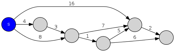
single-pair shortest path problem
Problem: Given a digraph \(G = (V,E)\), edge lengths \(l_e \geq 0\), source \(s \in V\), and destination \(t \in V\), find a shortest directed path from \(s\) to \(t\).
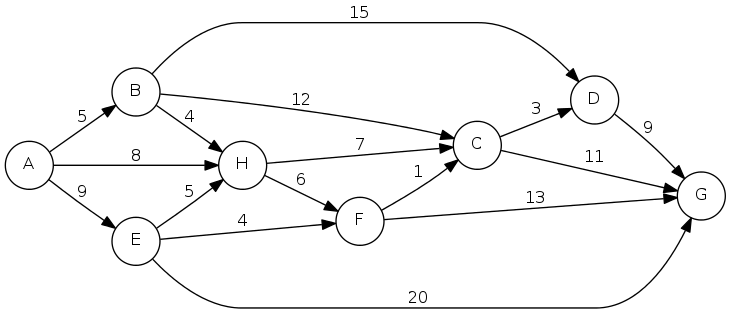
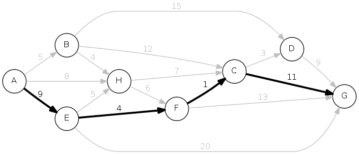
Length of path: \(9 + 4 + 1 + 11 = 25\)
Assumption: there exists a path from \(s\) to every node
quiz 7: greedy algorithms
Suppose that you change the length of every edge of \(G\) as follows to create a new graph \(G'\). For which is every shortest path in \(G\) a shortest path in \(G'\)?
-
\(l'_e = l_e + 17\) (Add 17)
-
\(l'_e = 17 \cdot l_e\) (Multiply by 17)
-
Both A and B
-
Neither A nor B
quiz 8: greedy algorithms

Which variant in car GPS?
-
Single source: from one node \(s\) to every other node
-
Single sink: from every node to one node \(t\)
-
Source-sink: from one node \(s\) to another node \(t\)
-
All pairs: between all pairs of nodes
shortest path applications
- PERT / CPM
- map routing
- seam carving
- robot navigation
- texture mapping
- typesetting in \(\LaTeX\)
- urban traffic planning
- telemarketer operator scheduling
- routing of telecommunications messages
- network routing protocols (OSPF, BGP, RIP)
- optimal truck routing through given traffic congestion pattern
shortest path applications
Dijkstra's alg (for single-source shortest paths problem)
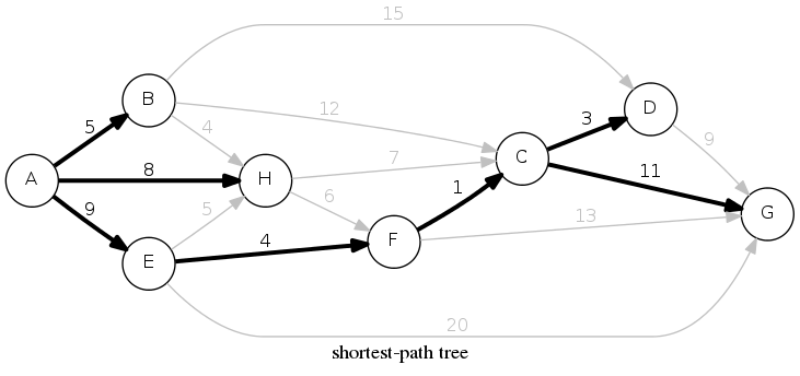
Greedy approach: Maintain a set of explored nodes \(S\) for which algorithm has determined \(d[u]\) as length of a shortest \(s {\leadsto} u\) path.
- Initialize \(S \leftarrow \{ s \}, d[s] \leftarrow 0\)
- Repeatedly choose unexplored node \(v \notin S\) which minimizes
\[ \pi(v) = \min_{e=(u,v):u\in S} d[u] + l_e \]
where \(d[u]+l_e\) is the length of a shortest path from \(s\) to some node \(u\) in explored part \(S\), followed by a single edge \(e=(u,v)\)
- add \(v\) to \(S\) and set \(d[v] \leftarrow \pi(v)\)
- to recover path, set \(\mathrm{pred}[v] \leftarrow e\) that achieves min
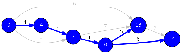
group: Dijkstra's alg: Demo
- Initialize \(S \leftarrow \{s\}\) and \(d[s] \leftarrow 0\)
- Repeatedly choose unexplored node \(v \notin S\) which minimizes
\[ \pi(v) = \min_{e=(u,v):u \in S} d[u] + l_e \]
- add \(v\) to \(S\); set \(d[v] \leftarrow \pi(v)\) and \(\mathrm{pred}[v] \leftarrow e\), the \(\mathrm{argmin}\)
\(S\): blue nodes, \(\mathrm{pred}[v]\): blue arrow, \(\pi(v)\): node label
\(S\): blue nodes, \(\mathrm{pred}[v]\): blue arrow, \(\pi(v)\): node label
Dijkstra's alg: proof of correctness
Invariant: For each node \(u \in S\): \(d[u]\) is len of a shortest \(s {\leadsto} u\) path
Pf by induction on \(|S|\):
-
Base case: \(|S| = 1\) is easy since \(S = \{s\}\) and \(d[s]=0\)
-
Inductive hypothesis...
Dijkstra's alg: proof of correctness
Invariant: For each node \(u \in S\): \(d[u]\) is len of a shortest \(s {\leadsto} u\) path
- Inductive hypothesis: Assume true for \(|S| \geq 1\)
- Let \(v\) be next node added to \(S\) and \((u,v)\) be the final edge
- A shortest \(s {\leadsto} u\) path plus \((u,v)\) is an \(s {\leadsto} v\) path of len \(\pi(v)\)
- Consider any other \(s {\leadsto} v\) path \(P\). We show that it is no shorter than \(\pi(v)\).
- Let \(e=(x,y)\) be the first edge in \(P\) that leaves \(S\), and let \(P'\) be the subpath from \(s\) to \(x\)
- The length of \(P\) is already \(\geq \pi(v)\) as soon as it reaches \(y\):
\[ l(P) \geq^{*} l(P') + l_e \geq^{\dagger} d[x] + l_e \geq^{\ddagger} \pi(y) \geq^{\star} \pi(v) \]
where \(\geq^*\)non-negative lengths, \(\geq^\dagger\)inductive hypothesis,
\(\geq^\ddagger\)definition of \(\pi(y)\), \(\geq^\star\)Dijkstra chose \(v\) instead of \(y\) ∎
dijkstra's alg: efficient implementation
Critical optimization 1: For each unexplored node \(v \notin S\), explicitly maintain \(\pi[v]\) instead of computing directly from definition
\[ \pi(v) = \min_{e = (u,v): u \in S} d[u] + l_e \]
- For each \(v \notin S\): \(\pi(v)\) can only decrease (because set \(S\) increases)
- More specifically, suppose \(u\) is added to \(S\) and there is an edge \(e=(u,v)\) leaving \(u\). Then it suffices to update \[ \pi[v] \leftarrow \min \{ \pi[v], \pi[u] + l_e \} \] recall for each \(u \in S\), \(\pi[u] = d[u] =\) length of shortest \(s\leadsto u\) path
dijkstra's alg: efficient implementation
Critical optimization 1: For each unexplored node \(v \notin S\), explicitly maintain \(\pi[v]\) instead of computing directly from definition
Critical optimization 2: Use a min-oriented priority queue (MinPQ) to choose an unexplored node that minimizes \(\pi[v]\)
dijkstra's alg: efficient implementation
Implementation
- Algorithm maintains \(\pi[v]\) for each node \(v\)
- Priority queue stores unexplored nodes, using \(\pi[\cdot]\) as priorities
- Once \(u\) is deleted from the MinPQ, \(\pi[u]\) is length of a shortest \(s{\leadsto}u\) path
Dijkstra(V, E, l, s):
    ForEach v != s: pi[v] <- infty, pred[v] <- null
    pi[s] <- 0
    Create an empty priority queue pq
    ForEach v in V: Insert(pq, v, pi[v])
    While pq is not empty:
        u <- DelMin(pq)
        ForEach edge e=(u,v) in E leaving u:
            If pi[v] > pi[u] + l[e]
                DecreaseKey(pq, v, pi[u] + l[e])
                pi[v] <- pi[u] + l[e]
                pred[v] <- e
dijkstra's alg: which priority queue?
Performance depends on PQ: \(n\) insert, \(n\) del-min, \(\leq m\) dec-key
- Array implementation optimal for dense graphs (\(\Theta(n^2)\) edges)
- Binary heap much faster for sparse graphs (\(\Theta(n)\) edges)
- 4-way heap worth the trouble in performance-critical situations
| priority queue | insert | del-min | dec-key | total |
|---|---|---|---|---|
| unordered array | \(O(1)\) | \(O(n)\) | \(O(1)\) | \(O(n^2)\) |
| binary heap | \(O(\log n)\) | \(O(\log n)\) | \(O(\log n)\) | \(O(m \log n)\) |
| d-way heap | \(O(d \log_d n)\) | \(O(d \log_d n)\) | \(O(\log_d n)\) | \(O(m \log_\dagger n)\) |
| fibonacci heap | \(O(1)\) | \(O(\log n)^\ddagger\) | \(O(1)^\ddagger\) | \(O(m + n \log n)\) |
| integer pq | \(O(1)\) | \(O(\log \log n)\) | \(O(1)\) | \(O(m + n \log \log n)\) |
\(\dagger\) log base is \(m/n\), \(\ddagger\) amortized
quiz 9: greedy algorithms
How to solve the single-source shortest paths problem in undirected graphs with positive edge lengths?
-
Replace each undirected edge with two antiparallel edges of same length. Run Dijkstra's algorithm in the resulting digraph
-
Modify Dijkstra's algorithm so that when it processes node \(u\), it considers all edges incident to \(u\) (instead of edges leaving \(u\))
-
Both A and B
-
Neither A nor B
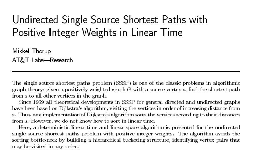
Dijkstra's alg: undirected graphs
Theorem [Thorup 1999]: Can solve single-source shortest paths problem in undirected graphs with positive integer edge lengths in \(O(m)\) time
Remark: Does not explore nodes in increasing order of distance from \(s\)
 |
 |
Extensions of Dijkstra's algorithm
Dijkstra's algorithm and proof extend to several related problems:
- Shortest paths in undirected graphs: \(\pi[v] \leq \pi[u] + l(u,v)\)
- Maximum capacity paths: \(\pi[v] \geq \min \{ \pi[u], c(u,v) \}\)
- Maximum reliability paths: \(\pi[v] \geq \pi[u] \times \gamma(u,v)\)
- ...
Key algebraic structure: Closed semiring (min-plus, bottleneck, Viterbi, ...) \[ \begin{array}{rcl} a+b & = & b+a \\ a + (b+c) & = & (a+b)+c \\ a + 0 & = & a \\ a \cdot (b \cdot c) & = & (a \cdot b) \cdot c \\ a \cdot 0 & = & 0 \cdot a = 0 \\ a \cdot 1 & = & 1 \cdot a = a \\ a \cdot (b + c) & = & a \cdot b + a \cdot c \\ (a + b) \cdot c & = & a \cdot c + b \cdot c \\ a^* = 1 + a\cdot a^* & = & 1 + a^* \cdot a \end{array}\]
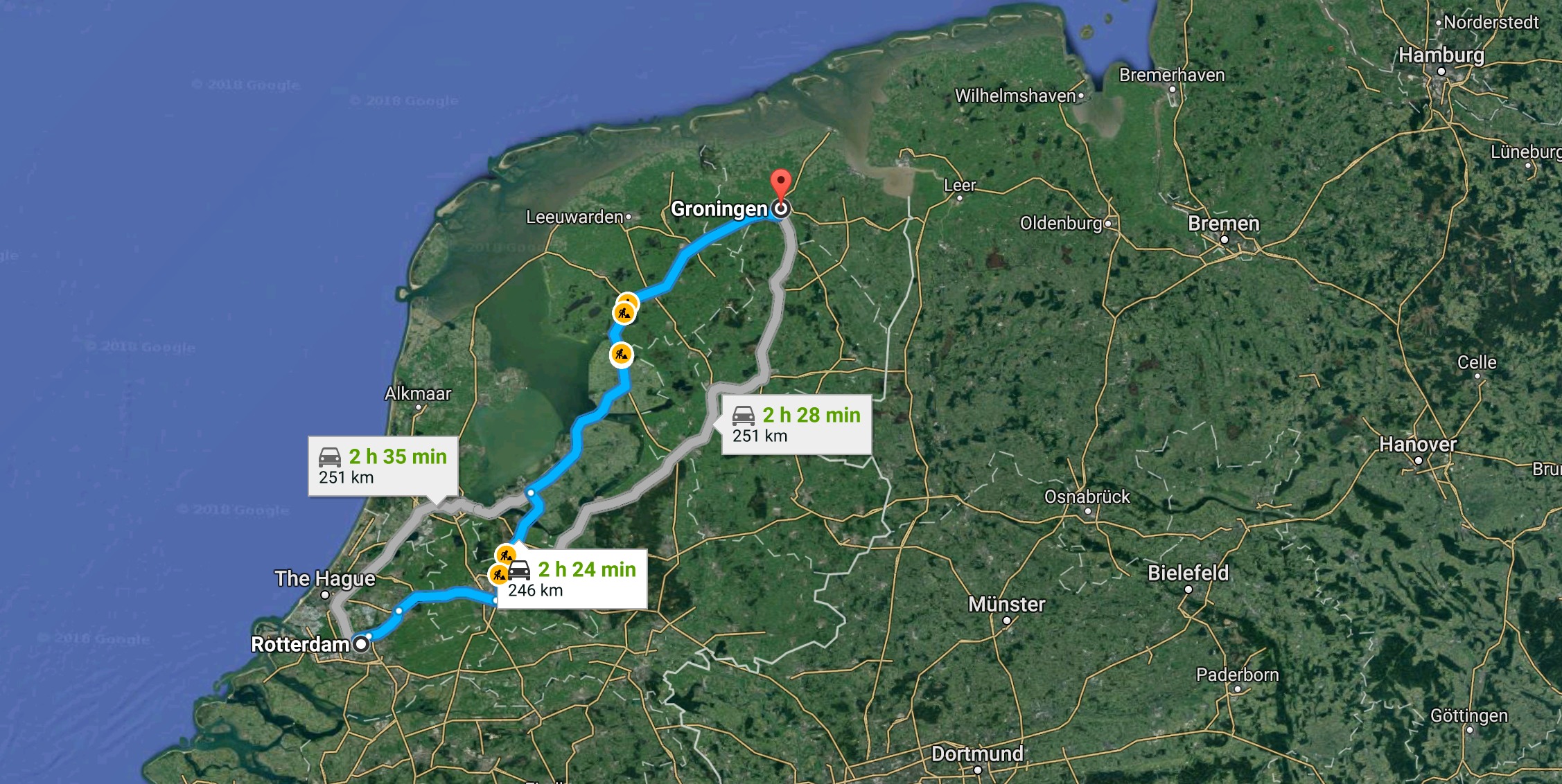
Edsger Dijkstra
“What's the shortest way to travel from Rotterdam to Groningen? It is the algorithm for the shortest path, which I designed in about 20 minutes. One morning I was shopping in Amsterdam with my young fiancée, and tired, we sat down on the café terrace to drink a cup of coffee and I was just thinking about whether I could do this, and I then designed the algorithm for the shortest path.
”
 |
 |
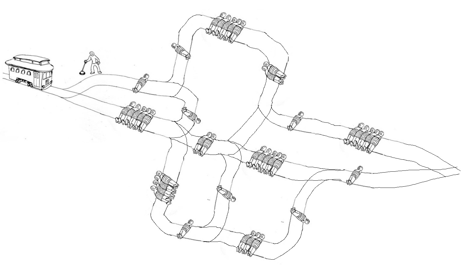
moral implications of shortest-path alg
Greedy Algorithms
Google's Foo.bar Challenge
Group: Google's foo.bar challenge
You have maps of parts of the space station, each starting at a prison exit
and ending at the door to an escape pod.  The map is represented as a matrix
of 0s and 1s, where 0s are passable space and 1s are impassable walls.  The
door out of the prison is at the top-left (0,0) and the door into an escape
pod is at the bottom-right (w - 1, h - 1).

Write a function that generates the length of a shortest path from the prison
door to the escape pod, where you are allowed to remove one wall as part of
your remodeling plans.
| s | ||||||||||||
| t |
Greedy Algorithms
minimum spanning trees (4.5)
paths and cycles
Defn: A path is a sequence of edges which connects a sequence of nodes.
Defn: A cycle is a path with no repeated nodes or edges other than the starting and ending nodes.
path \(P = \{ (1,2), (2,3), (3,4), (4,5), (5,6) \}\)
cycle \(C = \{ (1,2), (2,3), (3,4), (4,5), (5,6), (6,1) \}\)
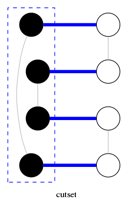
cuts and cut-sets
Defn: A cut is a partition of the vertices of a graph into two nonempty, disjoint subsets, \(S\) and \(V-S\)
Defn: The cut-set of a cut \(S\) is the set of edges with exactly one endpoint in \(S\)
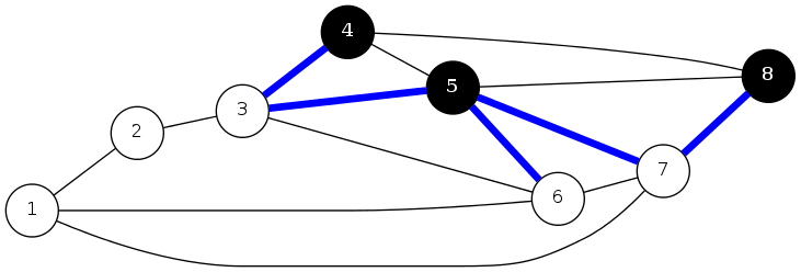
cut \(S = \{ 4, 5, 8 \}\)
cut-set \(D = \{ (3,4), (3,5), (5,6), (5,7), (8,7) \}\)
quiz 10: greedy algorithms
Consider the cut \(S = \{1,4,6,7\}\). Which edge is in cut-set of \(S\)?
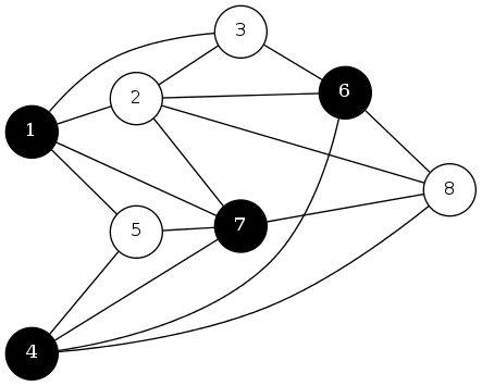
- \((5,7)\)
- \((1,7)\)
- \((2,3)\)
- \(S\) is not a cut (not connected)
quiz 11: greedy algorithms
Let \(C\) be a cycle and let \(D\) be a cut-set. How many edges do \(C\) and \(D\) have in common? Choose the best answer.
- 0
- 2
- not 1
- an even number
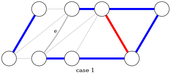
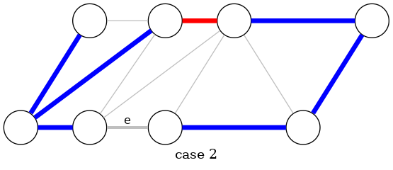
cycle-cut intersection
Proposition: A cycle and a cut-set intersect in an even number of edges
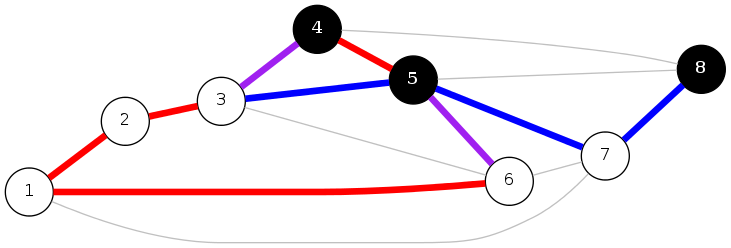
cycle \(C = \{ (1,2), (2,3), (3,4), (4,5), (5,6), (6,1) \}\)
cut-set \(D = \{ (3,4), (3,5), (5,6), (5,7), (7,8) \}\)
intersection \(C \cap D = \{ (3,4), (5,6) \}\)
cycle-cut intersection
Proposition: A cycle and a cut-set intersect in an even number of edges.
Pf by picture:
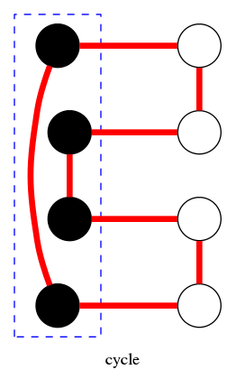 |
 |
spanning tree definition
Defn: Let \(H = (V,T)\) be a subgraph of an undirected graph \(G=(V,E)\). \(H\) is a spanning tree of \(G\) if \(H\) is both acyclic and connected.
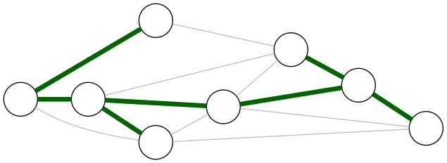
graph \(G = (V, E)\)
spanning tree \(H = (V,T)\)
note: \(H\) contains all vertices of \(G\); \(T \subseteq E\)
quiz 12: greedy algorithms
Which of the following properties are true for all spanning trees \(H\)?
-
Contains exactly \(|V|-1\) edges
-
The removal of any edge \(e \in T\) disconnects it
-
The addition of any other edge \(e \in E\) creates a cycle
-
All of the above.
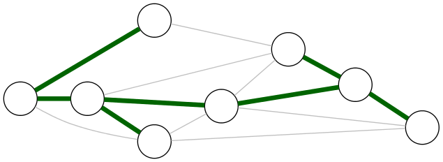
graph \(G = (V, E)\), spanning tree \(H = (V,T)\)
spanning tree properties
Proposition: Let \(H = (V,T)\) be a subgraph of an undirected graph \(G=(V,E)\). Then, the following are equivalent:
- \(H\) is a spanning tree of \(G\)
- \(H\) is acyclic and connected
- \(H\) is connected and has \(|V|-1\) edges
- \(H\) is acyclic and has \(|V|-1\) edges
- \(H\) is minimally connected: removal of any edge disconnects it
- \(H\) is maximally acyclic: addition of any edge creates a cycle
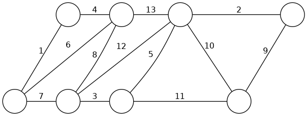
minimum spanning tree (MST)
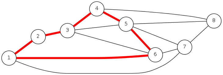
Defn: Given a connected, undirected graph \(G=(V,E)\) with edge costs \(c_e\), a minimum spanning tree \((V,T)\) is a spanning tree of \(G\) such that the sum of the edge costs in \(T\) is minimized.
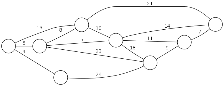
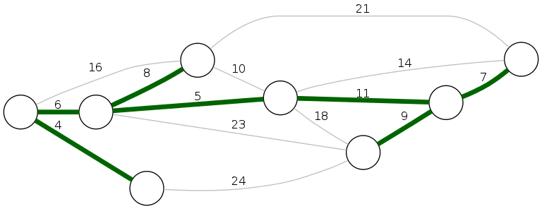
MST cost: \(4 + 6 + 8 + 5 + 11 + 9 + 7 = 50\)
Cayley's theorem: The complete graph on \(n\) nodes has \(n^{n-2}\) spanning trees (cannot solve by brute force)
quiz 13: greedy algorithms
Suppose that you change the cost of every edge in \(G\) as follows to create a new graph \(G'\). For which is every MST in \(G\) an MST in \(G'\) (and vice versa)? Assume \(c_e > 0\) for each \(e\).
-
\(c'_e = c_e + 17\)
-
\(c'_e = 17 \cdot c_e\)
-
\(c'_e = \log_{17} c_e\)
-
All of the above
applications
MST is fundamental problem with diverse applications
- dithering
- cluster analysis
- max bottleneck paths
- real-time face verification
- LDPC codes for error correction
- image registration with Renyi entropy
- find road networks in satellite and aerial imagery
- model locality of particle interactions in turbulent fluid flows
- reducing data storage in sequencing amino acids in a protein
- Autoconfig protocol for Ethernet bridging to avoid cycles in a network
- approx algorithms for NP-hard problems (e.g., TSP, Steiner tree)
- network design (communications, electrical, hydraulic, computer, road)
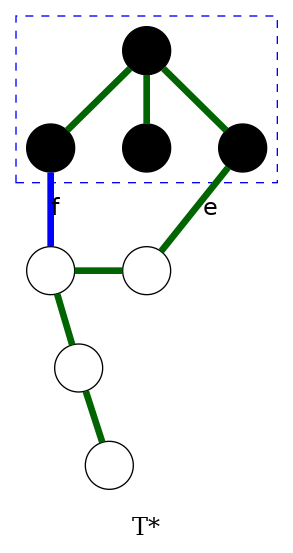
fundamental cycle
Fundamental cycle: Let \(H=(V,T)\) be a spanning tree of \(G=(V,E)\).
- For any non tree-edge \(e \in E-T\): \(T \cup \{ e \}\) contains a unique cycle, say \(C\)
- For any edge \(f \in C\): \(T \cup \{e\} - \{f\}\) is a spanning tree
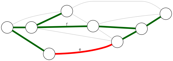
graph \(G = (V, E)\), spanning tree \(H = (V,T)\)
Observation: If \(c_e < c_f\), then \(H\) is not an MST
fundamental cut-set
Fundamental cut-set: Let \(H=(V,T)\) be a spanning tree of \(G=(V,E)\)
- For any tree edge \(f \in T\): \(T - \{f\}\) contains two connected components. Let \(D\) denote corresponding cut-set
- For any edge \(e \in D\): \(T - \{f\} \cup \{e\}\) is a spanning tree.
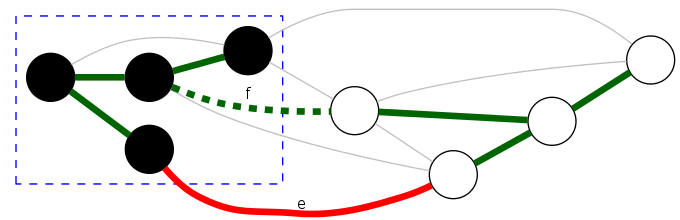
graph \(G = (V, E)\), spanning tree \(H = (V,T)\)
Observation: If \(c_e < c_f\), then \(H\) is not an MST.
the greedy algorithm
Red rule:
- Let \(C\) be a cycle with no red edges
- Select an uncolored edge of \(C\) of max cost and color it red
Blue rule:
- Let \(D\) be a cut-set with no blue edges
- Select an uncolored edge in \(D\) of min cost and color it blue
Greedy Algorithm:
- Apply the red and blue rules (nondeterministically) until all edges are colored. The blue edges form an MST
- Note: can stop once \(n-1\) edges colored blue
the greedy algorithm
- Apply nondeterministically until all edges are colored
- Find cycle with no red edges. Color red the uncolored edge with max cost
- Find cut-set with no blue edges. Color blue the uncolored edge with min cost
- blue edges form an MST
greedy algorithm: proof of correctness
Color invariant: There exists an MST \((V,T^*)\) containing every blue edge and no red edge.
Pf by induction on number of iterations:
Base case: no edges colored ⇒ every MST satisfies invariant.
greedy algorithm: proof of correctness
Color invariant: There exists an MST \((V,T^*)\) containing every blue edge and no red edge.
Pf by induction on number of iterations:
Inductive step (blue): Suppose color invariant true before blue rule
- Let \(D\) be chosen cut-set, and let \(f\) be edge colored blue
- If \(f \in T^*\), then \(T^*\) still satisfies invariant
- Otherwise, consider fundamental cycle \(C\) by adding \(f\) to \(T^*\)
- Let \(e \in C\) be another edge in \(D\)
- \(e\) is uncolored and \(c_e \geq c_f\) since
- \(e \in T^*\) ⇒ \(e\) not red
- blue rule ⇒ \(e\) not blue and \(c_e \geq c_f\)
- Thus, \(T^* \cup \{f\} - \{e\}\) satisfies invariant
greedy algorithm: proof of correctness
Color invariant: There exists an MST \((V,T^*)\) containing every blue edge and no red edge.
Pf by induction on number of iterations:
Inductive step (red): Suppose color invariant true before red rule

- Let \(C\) be chosen cycle, and let \(e\) be edge colored red
- If \(e \notin T^*\), then \(T^*\) still satisfies invariant
- Otherwise, consider fundamental cut-set \(D\) by deleting \(e\) from \(T^*\)
- Let \(f \in D\) be another edge in \(C\)
- \(f\) is uncolored and \(c_e \geq c_f\) since
- \(f \notin T^*\) ⇒ \(f\) not blue
- red rule ⇒ \(f\) not red and \(c_e \geq c_f\)
- Thus, \(T^* \cup \{f\} - \{e\}\) satisfies invariant ∎
greedy algorithm: proof of correctness
Theorem: The greedy algorithm terminates. Blue edges form MST
Pf: We need to show that either the red or blue rule (or both) applies
- Suppose edge \(e\) is left uncolored.
- Blue edges form a forest
- Case 1: Both endpoints of \(e\) are in same blue tree
- ⇒ apply red rule to cycle formed by adding \(e\) to blue forest
greedy algorithm: proof of correctness
Theorem: The greedy algorithm terminates. Blue edges form MST
Pf: We need to show that either the red or blue rule (or both) applies
- Suppose edge \(e\) is left uncolored.
- Blue edges form a forest
- Case 2: Endpoints of \(e\) are in different blue trees
- ⇒ apply blue rule to cut-set induced by either of two blue trees. ∎
Greedy Algorithms
prim, kruskal, reverse-delete (4.6)
prim's algorithm
- Initialize \(S\) as any node, \(T = \emptyset\)
- Repeat \(n-1\) times
- Add to \(T\) a min-cost edge with one endpoint in \(S\)
- Add new node to \(S\)
Theorem: Prim's algorithm computes an MST
Pf: Special case of greedy algorithm, where blue rule repeatedly applied to \(S\) (By construction, edges in cut-set are uncolored) ∎
prim's algorithm: implementation
Theorem: Prim's algorithm can be implemented to run in \(O(m \log n)\) time
Pf: Implementation almost identical to Dijkstra's algorithm
Prim(V, E, c):
    S <- {}, T <- {}
    s <- any node in V
    Foreach v != s: pi[v] <- infty, pred[v] <- null; pi[s] <- 0
    Create an empty minimum priority queue pq
    Foreach v in V: Insert(pq, v, pi[v])
    While Is-Not-Empty(pq):
        u <- Del-Min(pq)
        S <- Union(S, { u }), T <- Union(T, { pred[u] })
        Foreach edge e = (u,v) in E with v notin S:
            If c[e] < pi[v]:
                Decrease-Key(pq, v, c[e])
                pi[v] <- c[e]; pred[v] <- e
    Return T
Kruskal's Algorithm
Consider edges in ascending order of cost: Add to tree unless it would create a cycle
Theorem: Kruskal's algorithm computes an MST
Pf: Special case of greedy algorithm
- Case 1: both endpoints of \(e\) in same blue tree
- ⇒ color \(e\) red by applying red rule to unique cycle (all other edges in cycle are blue)
- Case 2: endpoints of \(e\) in different blue trees
- ⇒ color \(e\) blue by applying blue rule to cut-set defined by either tree. (no edge in cut-set has smaller cost since Kruskal chose it first) ∎
kruskal's algorithm: implementation
Theorem: Kruskal's algorithm can be implemented to run in \(O(m \log m)\) time.
- Sort edges by cost in ascending order
- Use union-find data structure to dynamically maintain connected components
Kruskal(V, E, c):
    Sort m edges by cost and renumber so that c[e1] <= c[e2] <= ... <= c[em]
    T <- {}
    Foreach v in V: UF-Make-Set(v)
    For i = 1 to m:
        (u,v) <- ei
        If UF-Find(u) != UF-Find(v): // u and v in diff components
            T <- Union(T, {ei})
            UF-Union(u, v)           // make u and v in same component
    Return T
reverse-delete algorithm
- Start with all edges in \(T\) and consider them in descending order of cost
- Delete edge from \(T\) unless it would disconnect \(T\)
Theorem: The reverse-delete algorithm computes an MST
Pf: Special case of greedy algorithm
- Case 1: Deleting edge \(e\) does not disconnect \(T\)
- ⇒ apply red rule to cycle \(C\) formed by adding \(e\) to another path in \(T\) between its two endpoints (no edge in \(C\) is more expensive; it would have already been considered and deleted)
reverse-delete algorithm
- Start with all edges in \(T\) and consider them in descending order of cost
- Delete edge from \(T\) unless it would disconnect \(T\)
Theorem: The reverse-delete algorithm computes an MST
Pf: Special case of greedy algorithm
- Case 2: Deleting edge \(e\) disconnects \(T\)
- ⇒ apply blue rule to cut-set \(D\) induced by either component (\(e\) is the only remaining edge in the cut-set; all other edges in \(D\) must have been colored red / deleted) ∎
Fact: [Thorup 2000] Can be implemented to run in \(O(m \log n (\log \log n)^3)\) time
review: the greedy mst algorithm
Red rule:
- Let \(C\) be a cycle with no red edges
- Select an uncolored edge of \(C\) of max cost and color it red
Blue rule:
- Let \(D\) be a cut-set with no blue edges
- Select an uncolored edge in \(D\) of min cost and color it blue
Greedy Algorithm:
- Apply the red and blue rules (nondeterministically) until all edges are colored. The blue edges form an MST
- Note: can stop once \(n-1\) edges colored blue
Theorem: the greedy algorithm is correct.
Special cases: Prim, Kruskal, reverse-delete, ...
group: Find MST of graph
Prim: add any node to \(S\), repeat \(n-1\) times: find min-cost edge with one endpoint in \(S\), add other node to \(S\)
Kruskal: sort edges in inc order, add to tree unless it creates cycle
Reverse-delete: all edges in "tree", sort edges in dec order, del edge from tree unless it would disconnect tree