Analysis of Algorithms
COS 265 - Data Structures & Algorithms
Analysis of Algorithms
introduction
cast of characters
-
Programmer needs to develop a working solution
-
Client wants to solve problem efficiently
-
Theoretician seeks to understand
Although you all are currently students, someday you might play any or all of these roles
running time
“As soon as an Analytical Engine exists, it will necessarily guide the future course of the science. Whenever any result is sought by its aid, the question will then arise—By what course of calculation can these results be arrived at by the machine in the shortest time?
”
–Charles Babbage (1864)

running time
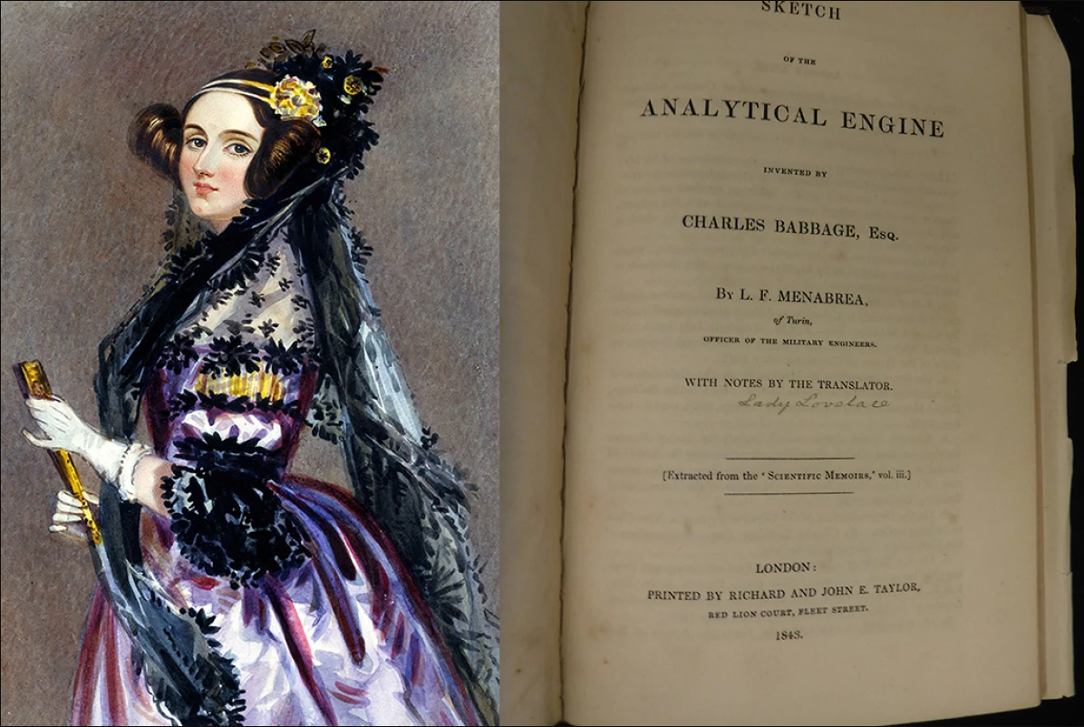
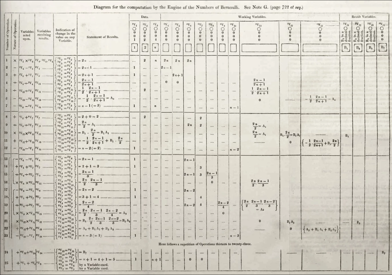
“Rare book containing the world’s first computer algorithm earns $125,000 at auction
”
Ada Lovelace's algorithm to compute Bernoulli numbers on Analytical Engine (1843)
 |
 |
reasons to analyze algorithms
- Predict performance *
- Compare algorithms *
- Provide guarantees *†
- Understand theoretical basis †
Primary practical reason: avoid performance bugs
Client gets poor performance because programmer did not understand performance characteristics
| * | COS 265 Data Structures and Algorithms |
| † | COS 320 Algorithm Design, COS 435 Theory of Computation |
an algorithmic success story
N-body simulation
- Simulate gravitational interactions among \(N\) bodies
- Applications: cosmology, fluid dynamics, semiconductors, ...
- Brute force: \(N^2\) steps
- Barnes-Hut algorithm: \(N \log N\) steps, enabling new research
 |
|
an algorithmic success story
Discrete Fourier transform
- Express signal as weighted sum of sines and cosines
- Applications: DVD, JPEG, MRI, astrophysics, ...
- Brute force: \(N^2\) steps
- FFT algorithm: \(N \log N\) steps, enabling new technology

the challenge
Q: Will my program be able to solve a large practical input?
“Why is my program so slow??
”
“Why does it run out of memory??
”
Insight by Knuth (1970s): Use scientific method to understand performance
scientific method applied to alg. analysis
A framework for predicting performance and comparing algorithms
Scientific method:
- Observe some feature of the natural world
- Hypothesize a model that is consistent with the observations
- Predict events using the hypothesis
- Verify the predictions by making further observations
- Validate by repeating until the hypothesis and observations agree
Principles:
- Experiments must be reproducible
- Hypotheses must be falsifiable
algorithm analysis
observations
example: 3-sum
3-Sum: Given \(N\) distinct integers, how many triples sum to exactly zero?
Context: Deeply related to problems in computational geometry
$ cat 8ints.txt 8 30 -40 -20 -10 40 0 10 5 $ java ThreeSum 8ints.txt 4 |
|

3-sum brute-force algorithm
ThreeSum.java: source, 1Kints.txt, 2Kints.txt, 4Kints.txt, 8Kints.txt
public class ThreeSum {
    public static int count(int[] a) {
        int N = a.length;
        int count = 0;

        // check each triple (ignore integer overflow for simplicity)
        for(int i = 0; i < N; i++)
            for(int j = i+1; j < N; j++)
                for(int k = j+1; k < N; k++)
                    if(a[i] + a[j] + a[k] == 0)
                        count++;
        return count;
    }

    public static void main(String[] args) {
        In in = new In(args[0]);
        int[] a = in.readAllInts();
        StdOut.println(count(a));
    }
}
quiz: 3-sum brute-force run-time estimation
Based on the code listing to the right (same as previous slide), which of the following best estimates the run-time of running the brute force implementation of 3-sum?
int count(int[] a) {
    int N = a.length;
    int count = 0;

    // check each triple
    // ignore integer overflow for simplicity
    for(int i = 0; i < N; i++)
        for(int j = i+1; j < N; j++)
            for(int k = j+1; k < N; k++)
                if(a[i] + a[j] + a[k] == 0)
                    count++;
    return count;
}
- Constant
(independent of \(N\)) - \(N\)
- \(N^2\)
- \(N^3\)
measuring the running time
Q: How to time a program?
measuring the running time
Q: How to time a program?
A1: (ノಠ益ಠ)ノ Manually using a stopwatch
measuring the running time
Q: How to time a program?
A1: (ノಠ益ಠ)ノ Manually using a stopwatch
A2: (ಠ_ಠ) Using time Unix command (time java ThreeSum ...)
measuring the running time
Q: How to time a program?
A1: (ノಠ益ಠ)ノ Manually using a stopwatch
A2: (ಠ_ಠ) Using time Unix command (time java ThreeSum ...)
A3: (♥‿♥) Automatically using programming!

public static void main(String[] args) {
    In in = new In(args[0]);      // do "unimportant" stuff first
    int[] a = in.readAllInts();   // that should not be timed...

    Stopwatch stopwatch = new Stopwatch();    // start stopwatch
    StdOut.println(ThreeSum.count(a));        // run experiment
    double time = stopwatch.elapsedTime();    // record elapsed time

    StdOut.println("elapsed time = " + time);
}
Emperical analysis
Run the program for various input sizes and measure running time
| \(N\) | \(T(N)\) |
|---|---|
| 250 | 0.0 |
| 500 | 0.0 |
| 1000 | 0.1 |
| 2000 | 0.8 |
| 4000 | 6.4 |
| 8000 | 51.1 |
| 16000 | ??? |
\(T(N)\) is time in seconds on some particular machine
data analysis
Standard linear plot: \(T(N)\) vs. \(N\)

\(T(N)\): running time. \(N\): input size.
data analysis
Log-log plot: \(\log(T(N))\) vs. \(\log(N)\) (log-log scale)

\(T(N)\): running time. \(N\): input size.
data analysis
Log-log plot: \(\log(T(N))\) vs. \(\log(N)\) (log-log scale)
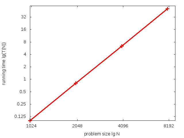 |
Line Equation: \(y = mx + b\) substitute for \(y\),\(x\) and solve for \(m\),\(b\) \(\underbrace{\lg(T(N))}_y = m \cdot \underbrace{\lg N}_x + b\) Fit line to data using regression: |
Power Law Equation: \(T(N) = a N^b\)
Hypothesis: Running time is about \(1.006\cdot10^{-10} \times N^{2.999}\) secs
Note
\(a\) in power law is equal to \(2^b\), where \(b\) is from line equation.
prediction and validation
Hypothesis: Running time is about \(1.006 \cdot 10^{-10} \times N^{2.999}\) secs
("order of growth" of running time is about \(N^3\))
|
Predictions:
|
Observations:
|
Observations validate hypothesis!
doubling hypothesis
Doubling hypothesis: Quick way to estimate \(b\) in a power-law relationship
Run program, doubling the size of the input
|
\[\frac{T(N)}{T(N/2)} = \frac{aN^b}{a(N/2)^b} = 2^b\] \[\lg (6.4 / 0.8) = 3.0\] seems to converge to \(b \approx 3\) |
Hypothesis: Running time is about \(aN^b\) with \(b = \lg \text{ratio}\)
Note
Caveat: Cannot identify log factors with doubling hypothesis (ex: \(N \lg N\))
doubling hypothesis
Q: How to estimate \(a\) (assuming we know \(b\))?
A: Run the program (for sufficiently large value of \(N\)) and solve for \(a\)
\(b \approx 3\) from prev slide |
\[\begin{array}{rcl} a N^b & = & T(N) \\ a \times 8000^3 & = & 51.1 \\ a &= & 0.998 \cdot 10^{-10} \end{array}\] |
Hypothesis: Running time is about \(0.998 \cdot 10^{-10} \times N^3\) seconds
Note: this is almost identical hypothesis to one obtained via regression (\(1.006 \cdot 10^{-10} \times N^{2.999}\)), but required less work and can write code to compute this!
math tangent: change of base
Most math libraries do not have \(\lg = \log_2\) function
But you can compute \(\log\) of \(A\) with any base \(b\) using the \(\log\) of any other base
\[ \log_b A = \frac{\log_c A}{\log_c b} \]
So, if you have \(\log_{10}\) (Math.log10) or \(\ln = \log_e\) (Math.log), you can compute \(\lg\) as
\[ \log_2 A = \frac{\log_{10} A}{\log_{10} 2} = \frac{\ln A}{\ln 2} \]
quiz: estimate running time
Estimate the running time (\(T(N)\), units:seconds) to solve a problem of size \(N=96{,}000\) based on the timing table on right.
| \(N\) | \(T(N)\) |
|---|---|
| 1,000 | 0.02 |
| 2,000 | 0.05 |
| 4,000 | 0.20 |
| 8,000 | 0.81 |
| 16,000 | 3.25 |
| 32,000 | 13.01 |
| 96,000 | ???? |
- 39 seconds
- 52 seconds
- 117 seconds
- 350 seconds
experimental algorithmics
\[\text{power law: } \quad T(N) = a N^b\]
system independent effects, determines factor \(a\) and exponent \(b\)
- algorithm
- input data
system dependent effects, determines factor \(a\)
- hardware: CPU, memory, cache, ...
- software: compiler, interpreter, garbage collector, ...
- system: operating system, network, other apps, ...
- power management: plugged in, plugged out, ...
bad news: sometimes difficult to get precise measurements
good news: much easier and cheaper than other sciences
as an aside
Algorithmic experiments are virtually free by comparison with other sciences
 |
 |
 |
 |
Bottom line: no excuse for not running experiments to understand costs
Analysis of Algorithms
mathematical models
mathematical models for running time
total running time: sum of cost × frequency for all operations
- need to analyze program to determine set of operations
- cost depends on machine, compiler
- frequency depends on algorithm, input data
 |
 |
In principle, accurate mathematical models are available.
example: 1-sum
Q: How many instructions as a function of input size \(N\)?
int count = 0;
for(int i = 0; i < N; i++)
    if(a[i] == 0)               // <- N array accesses
        count++;
| operation | cost \(\dagger\) | frequency |
|---|---|---|
| variable declaration | \(0.4\text{ ns}\) | \(2\) |
| assignment statement | \(0.2\text{ ns}\) | \(2\) |
| less-than compare | \(0.2\text{ ns}\) | \(N+1\) |
| equal-to compare | \(0.1\text{ ns}\) | \(N\) |
| array access | \(0.1\text{ ns}\) | \(N\) |
| increment | \(0.1\text{ ns}\) | \(N\) to \(2N\) |
\[ (1.4 + 0.5N) \text{ ns} \quad\textrm{to}\quad (1.4 + 0.6N) \text{ ns} \]
\(\dagger\) representative estimates (with some poetic license)
example: 2-Sum
Q: How many instructions as a function of input size \(N\)?
int count = 0;
for(int i = 0; i < N; i++)
    for(int j = i+1; j < N; j++)
        if(a[i] + a[j] == 0)        // inner loop
            count++;
Q: How many times does inner loop body (i.e., if) repeat?
example: 2-Sum
Q: How many instructions as a function of input size \(N\)?
int count = 0;
for(int i = 0; i < N; i++)
    for(int j = i+1; j < N; j++)
        if(a[i] + a[j] == 0)        // inner loop
            count++;
Q: How many times does inner loop body (i.e., if) repeat?
Pf. by Carl Friedrich Gauss
\[\begin{array}{cccccccccccc} & T(N) & = & 0 & + & 1 & + & \ldots & + & (N-2) & + & (N-1) \\ + & T(N) & = & (N-1) & + & (N-2) & + & \ldots & + & 1 & + & 0 \\ \hline & 2T(N) & = & (N-1) & + & (N-1) & + & \ldots & + & (N-1) & + & (N-1) \\ \\ & & \Rightarrow & T(N) & = & N (N-1) / 2 \end{array}\]
Note: \(0 + 1 + 2 + \ldots + (N-1) = \frac{1}{2} N (N-1) = \binom{N}{2}\)
example: 2-Sum
Q: How many instructions as a function of input size \(N\)?
int count = 0;
for(int i = 0; i < N; i++)
    for(int j = i+1; j < N; j++)
        if(a[i] + a[j] == 0)        // inner loop
            count++;
| operation | cost | frequency |
|---|---|---|
| variable declaration | \(0.4\text{ ns}\) | \(N+2\) |
| assignment statement | \(0.2\text{ ns}\) | \(N+2\) |
| less-than compare | \(0.2\text{ ns}\) | \(\onehalf (N+1)(N+2)\) |
| equal-to compare | \(0.1\text{ ns}\) | \(\onehalf N(N-1)\) |
| array access | \(0.1\text{ ns}\) | \(N(N-1)\) |
| increment | \(0.1\text{ ns}\) | \(\small \onehalf(N^2{+}3N{+}2)\) to \(\small N^2{+}N{+}1\) |
Timing is tedious to count exactly:
\[ \left( 0.30 N^2 + 0.90 N + 1.5 \right) \text{ns} \quad\textrm{to}\quad \left( 0.35 N^2 + 0.85 N + 1.5 \right) \text{ns} \]
simplifying the calculations
How do we simplify this work, especially so that we can analyze more complex algorithms?
“It is convenient to have a measure of the amount of work involved in a computing process, even though it be a very crude one. We may count up the number of times that various elementary operations are applied in the whole process and then given them various weights. We might, for instance, count the number of additions, subtractions, multiplications, divisions, recording of numbers, and extractions of figures from tables. In the case of computing with matrices most of the work consists of multiplications and writing down numbers, and we shall therefore only attempt to count the number of multiplications and recordings.
”
–Alan Turing (1947)
simplification 1: cost model
Cost model: use some basic operation as a proxy for running time
int count = 0;
for(int i = 0; i < N; i++)
    for(int j = i+1; j < N; j++)
        if(a[i] + a[j] == 0)        // inner loop
            count++;
| operation | cost | frequency | |
|---|---|---|---|
| variable declaration | \(0.4\text{ ns}\) | \(N+2\) | |
| assignment statement | \(0.2\text{ ns}\) | \(N+2\) | |
| less-than compare | \(0.2\text{ ns}\) | \(\onehalf (N+1)(N+2)\) | |
| equal-to compare | \(0.1\text{ ns}\) | \(\onehalf N(N-1)\) | |
| array access | \(0.1\text{ ns}\) | \(N(N-1)\) | ⇐ |
| increment | \(0.1\text{ ns}\) | \(N(N+1)\) to \(N^2\) |
cost model = array accesses, we assume compiler/JVM do not optimize any array accesses away
simplification 2: tilde notation
- estimate running time (or memory) as a function of input size \(N\)
- ignore lower order terms
- when \(N\) is large, lower order terms are negligible
- when \(N\) is small, we don't care
| original: \(f(N)\) | tilde: \(g(N)\) |
|---|---|
| \(\onesixth N^3 + 20N + 16\) | \(\sim\onesixth N^3\) |
| \(\onesixth N^3 + 100N^2 + 56\) | \(\sim\onesixth N^3\) |
| \(\onesixth N^3 - \onehalf N^2 + \onethird N\) | \(\sim\onesixth N^3\) |
Note
Technical definition: \(f(N) \sim g(N)\) means
\[\lim_{N \rightarrow \infty} \frac{f(N)}{g(N)} = 1\]
simplification 2: tilde notation
- estimate running time (or memory) as a function of input size \(N\)
- ignore lower order terms
- when \(N\) is large, lower order terms are negligible
- when \(N\) is small, we don't care
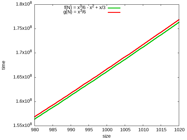 |
\[N = 1000\] \[f(N) = 166.17 \text{million}\] \[g(N) = 166.67 \text{million}\] |
simplification 2: tilde notation
- estimate running time (or memory) as a function of input size \(N\)
- ignore lower order terms
- when \(N\) is large, lower order terms are negligible
- when \(N\) is small, we don't care
| operation | frequency | tilde notation |
|---|---|---|
| var declaration | \(N+2\) | \(\sim N\) |
| assign statement | \(N+2\) | \(\sim N\) |
| less-than compare | \(\onehalf (N+1)(N+2)\) | \(\sim \onehalf N^2\) |
| equal-to compare | \(\onehalf N(N-1)\) | \(\sim \onehalf N^2\) |
| array access | \(N(N-1)\) | \(\sim N^2\) |
| increment | \(\onehalf N(N+1)\) to \(N^2\) | \(\sim \onehalf N^2\) to \(\sim N^2\) |
example: 2-Sum
Q: Approximately how many array accesses as a function of input size \(N\)?
int count = 0;
for(int i = 0; i < N; i++)
    for(int j = i+1; j < N; j++)
        if(a[i] + a[j] == 0)                // inner loop
            count++;
example: 2-Sum
Q: Approximately how many array accesses as a function of input size \(N\)?
int count = 0;
for(int i = 0; i < N; i++)
    for(int j = i+1; j < N; j++)
        if(a[i] + a[j] == 0)                // inner loop
            count++;
A: \(\sim N^2\) array accesses
Bottom line: use cost model and tilde notation to simplify counts
example: 3-sum
Q: Approximately how many array accesses as a function of input size \(N\)?
int count = 0;
for(int i = 0; i < N; i++)
    for(int j = i+1; j < N; j++)
        for(int k = j+1; k < N; k++)
            if(a[i] + a[j] + a[k] == 0)     // inner loop
                count++;
example: 3-sum
Q: Approximately how many array accesses as a function of input size \(N\)?
int count = 0;
for(int i = 0; i < N; i++)
    for(int j = i+1; j < N; j++)
        for(int k = j+1; k < N; k++)
            if(a[i] + a[j] + a[k] == 0)     // inner loop
                count++;
\[\binom{N}{3} = \frac{N(N-1)(N-2)}{3!} \sim \frac{1}{6}N^3\]
A: \(\sim \frac{1}{2} N^3\) array accesses
Bottom line: use cost model and tilde notation to simplify counts
Estimating a discrete sum
Q: How to estimate a discrete sum?
Estimating a discrete sum
Q: How to estimate a discrete sum?
A1: Take a discrete mathematics course (MAT 215)
Estimating a discrete sum
Q: How to estimate a discrete sum?
A1: Take a discrete mathematics course (MAT 215)
A2: Replace the sum with an integral and use calculus
Ex1: \(1 + 2 + \ldots + N\)
\[\sum_{i=1}^N i \sim \int_{x=1}^N x\ dx \sim \frac{1}{2}N^2\]
Estimating a discrete sum
Q: How to estimate a discrete sum?
A1: Take a discrete mathematics course (MAT 215)
A2: Replace the sum with an integral and use calculus
Ex2: \(1 + 1/2 + 1/3 + \ldots + 1/N\)
\[\sum_{i=1}^N \frac{1}{i} \sim \int_{x=1}^N \frac{1}{x}\ dx \sim \ln N\]
Estimating a discrete sum
Q: How to estimate a discrete sum?
A1: Take a discrete mathematics course (MAT 215)
A2: Replace the sum with an integral and use calculus
Ex3: 3-Sum triple loop
\[\sum_{i=1}^N \sum_{j=i}^N \sum_{k=j}^N 1 \sim \int_{x=1}^N \int_{y=x}^N \int_{z=y}^N dz\ dy\ dx \sim \frac{1}{6} N^3\]
Estimating a discrete sum
Q: How to estimate a discrete sum?
A1: Take a discrete mathematics course (MAT 215)
A2: Replace the sum with an integral and use calculus
Ex4: \(1 + 1/2 + 1/4 + 1/8 + \ldots\)
\[\sum_{i=0}^\infty \left(\frac{1}{2}\right)^i = 2\]
\[\int_{x=0}^\infty \left(\frac{1}{2}\right)^x\ dx = \frac{1}{\ln 2} \approx 1.4427\]
note: integral trick does not always work
Estimating a discrete sum
Q: How to estimate a discrete sum?
A1: Take a discrete mathematics course (MAT 215)
A2: Replace the sum with an integral and use calculus
A3: Use Maple or Wolfram Alpha

mathematical models for running time
In principle, accurate mathematical models are available.
In practice,
- Formulas can be complicated
- Advanced mathematics might be required
- Exact models best left for experts
mathematical models for running time
\[\begin{array}{ccl} T_N & = & c_1 A + c_2 B + c_3 C + c_4 D + c_5 E \\ A & = & \text{array access} \\ B & = & \text{integer add} \\ C & = & \text{integer compare} \\ D & = & \text{increment} \\ E & = & \text{variable assignment} \\ A–E & = & \text{frequencies (depend on algorithm, input)} \\ c_i & = & \text{costs (depend on machine, compiler)} \end{array}\]
Bottom line: we use approximate models in this course
\[T(N) \sim a N^b\]
analysis of algorithms
order-of-growth classifications
common order-of-growth classifications
Definition: If \(f(N) \sim c g(N)\) for some constant \(c > 0\), then the order of growth of \(f(N)\) is \(g(N)\).
- ignores leading coefficients
- ignores lower-order terms
Ex: The order of growth of the running time of this code is \(N^3\)
int count = 0;
for(int i = 0; i < N; i++)
    for(int j = i+1; j < N; j++)
        for(int k = j+1; k < N; k++)
            if(a[i] + a[j] + a[k] == 0)
                count++;
Typical usage: mathematical analysis of running times, where leading coefficients depend on machine, compiler, JVM, ...
common order-of-growth classifications
Good news: the set of functions below suffices to describe the order of growth of most common algorithms.
| constant | logarithmic | linear | linearithmic | quadratic | cubic | exponential |
|---|---|---|---|---|---|---|
| \(1\) | \(\log N\) | \(N\) | \(N \log N\) | \(N^2\) | \(N^3\) | \(2^N\) |

common order-of-growth classifications
| order | name | description | example | \(T(2N)/T(N)\) |
|---|---|---|---|---|
| \(1\) | constant | statement | add two numbers | \(1\) |
| \(\log N\) | logarithmic | divide in half | binary search | \(\sim 1\) |
| \(N\) | linear | single loop | find the max | \(2\) |
| \(N \log N\) | linearithmic | divide and conquer | mergesort | \(\sim 2\) |
| \(N^2\) | quadratic | double loop | check all pairs | \(4\) |
| \(N^3\) | cubic | triple loop | check all triples | \(8\) |
| \(2^N\) | exponential | exhaustive search | check all subsets | \(T(N)\) |
binary search
Goal: given a sorted array and a key, find index of the key in the array.
Binary search: compare key against middle entry
- too small: go left, repeat
- too big: go right, repeat
- equal: found it!
- else: cannot find it!
//          0  1  2  3  4  5  6  7  8  9 10 11 12 13 14
int[] a = {11,13,14,25,33,43,51,53,64,72,84,93,95,96,97};
binary search
| compare | >: left |
==: found it! |
a[mid] to key |
<: right |
empty: not in |
binary search: implementation
Trivial to implement?
binary search: implementation
Trivial to implement?
- First binary search published in 1946
- First bug-free one in 1962
- Bug in Java's
Arrays.binarySearch()discovered in 2006

binary search: java implementation
Invariant: if key appears in array a[], then a[lo]<=key<=a[hi].
public static int binarySearch(int key, int[] a) {
    int lo = 0, hi = a.length - 1;
    while(lo <= hi) {
        int mid = lo + (hi - lo) / 2;         // why not mid = (lo + hi) / 2?

        if     (key < a[mid]) hi = mid - 1;   // |
        else if(key > a[mid]) lo = mid + 1;   // | one "3-way compare"
        else return mid;                      // |
    }
    return -1;
}
binary search: mathematical analysis
Proposition: binary search uses at most \(1 + \lg N\) key compares to search a sorted array of size \(N\).
Def: \(T(N) =\) number key compares to binary search a sorted subarray of size \(\leq N\)
Binary search recurrence:
- \(T(N) \leq 1 + T(N/2)\) for \(N>1\)
- with \(T(1) = 1\)
binary search: mathematical analysis
Proposition: binary search uses at most \(1 + \lg N\) key compares to search a sorted array of size \(N\).
Pf sketch (assume \(N\) is a power of \(2\)) \[\begin{array}{rcll} T(N) & \leq & 1 + \quad\quad T(N/2) & \text{given} \\ & \leq & 1 + (1 + \quad T(N/4)) & \text{apply recurrence to 1st term} \\ & \leq & 1 + (1 + (1 + T(N/8))) & \text{apply recurrence to 1st term} \\ & \vdots & \vdots & \vdots \\ & \leq & \underbrace{1 + \ldots + 1}_{\lg N} + T(N/N) & \text{stop applying, } T(1)=1 \\ & = & \lg N + 1 & \end{array}\]
the 3-sum problem
3-Sum: Given \(N\) distinct integer, find three such that \(a + b + c = 0\)
-
Ver0: \(N^3\) time, \(N\) space
-
Ver1: \(N^2 \log N\) time, \(N\) space
-
Ver2: \(N^2\) time, \(N\) space
Note
For full credit in COS265, running time should be worst case.
Comparing programs
Hypothesis: the sorting-based \(N^2 \log N\) algorithm for 3-Sum is significantly faster in practice than the brute-force \(N^3\) algorithm.
|
|
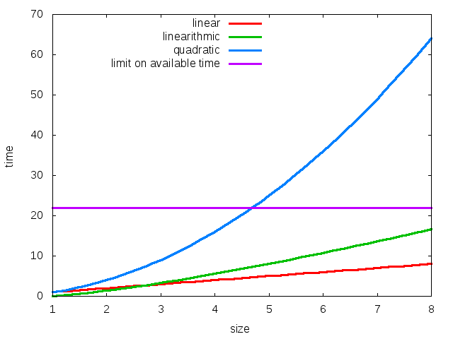
Guiding principle: Typically, better order of growth \(\Rightarrow\) faster in practice
Analysis of Algorithms
Memory
basics
| name | values/sizes | base |
|---|---|---|
| Bit | 0 or 1 |
binary |
| Byte | 8 bits | binary |
| Megabyte (MB) | 10002 bytes | decimal |
| Mebibyte (MiB) | 220 bytes | binary |
| Gigabyte (GB) | 10003 bytes | decimal |
| Gibibyte (GiB) | 230 bytes | binary |
64-bit machine: We assume a 64-bit machine with 8-byte pointers
(some JVMs "compress" ordinary object pointers to 4 bytes to avoid this cost)
Old school floppy disks: MB = 1000 * 1024 bytes (3.5" 1.44MB)
typical memory usage
typical memory usage for primitive types and one- and two-dimensional arrays
|
|
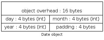
typical memory for Java objects
Each Java object
| Overhead | 16 bytes |
| Reference | 8 bytes |
| Padding | round up to 8 bytes |
Each object uses a multiple of 8 bytes
Ex: A Date object uses 32 bytes of memory
public class Date {
    private int day;
    private int month;
    private int year;
    // ...
}
|
 |
typical memory usage summary
Total memory usage for a data type value:
| Primitive | \(4\) bytes for int, \(8\) bytes for double, ... |
| Object ref | \(8\) bytes |
| Enum ref | \(8\) bytes |
| Array | \(24\) bytes + memory for each array entry |
| Object | \(16\) bytes + memory for each instance variable |
| (add \(8\) extra bytes if inner class object for reference to enclosing object) | |
| Padding | round up to multiple of \(8\) bytes |
Note
Depending on application, we may want to count memory for any referenced objects (recursively)
quiz: Analysis of algorithms
How much memory does a WeightedQuickUnionUF use as a function of \(N\)?
|
A: \(\sim 4N\) bytes B: \(\sim 8N\) bytes C: \(\sim 4N^2\) bytes D: \(\sim 8N^2\) bytes |
public class WeightedQuickUnionUF {
    private int[] parent;
    private int[] size;
    private int count;

    public WeightedQuickUnionUF(int N)
    {
        parent = new int[N];
        size = new int[N];
        count = 0;
        // ...
    }

    // ...
}
|
turning the crank: summary
Empirical analysis
- ...
Mathematical analysis
- ...
Scientific method
- ...
turning the crank: summary
Empirical analysis
- Execute program to perform experiments
- Assume power law
- Formulate a hypothesis for running time
- Model enables us to make predictions
Mathematical analysis
- ...
Scientific method
- ...
turning the crank: summary
Empirical analysis
- Execute program to perform experiments
- Assume power law
- Formulate a hypothesis for running time
- Model enables us to make predictions
Mathematical analysis
- Analyze algorithm to count frequency of operations
- Use tilde notation to simplify analysis
- Model enables us to explain behavior
Scientific method
- Mathematical model is independent of a particular system; applies to machine not yet built
- Empirical analysis is necessary to validate mathematical models and to make predictions